Electronic structure of 2D carbon materials#
Perfect graphene#
First we will investigate some of the basic properties of the 2D graphene structure.
Geometry, density of states#
[Input: recipes/defect/carbon2d-elect/graphene/latopt/]
Preparing the input#
Graphene has a hexagonal lattice with two C atoms in its primitive unit cell, which is specified in the supplied GEN-formatted geometry file. Open the file geo.gen in a text editor. You should see the following content:
2  S
C
 1 1    0.1427557522E+01    0.0000000000E-00    0.0000000000E-00
 2 1   -0.1427557522E+01    0.0000000000E-00    0.0000000000E-00
 0.0000000000E+00    0.0000000000E+00    0.0000000000E+00
 0.2141036415E+01   -0.1236340643E+01    0.0000000000E-00
 0.2141036415E+01    0.1236340643E+01    0.0000000000E-00
 0.0000000000E-00    0.0000000000E-00    0.5000000000E+02
Since the structure is periodic, appropriate information for this boundary condition must be provided after the atomic coordinates. For a GEN file of type
S, this is the cartesian coordinates of the origin followed by the 3 cartesian lattice vectors (one per line). DFTB+ uses three dimensional periodic boundary conditions. In order to separate the graphene sheets from each other and to prevent interaction between them, the third lattice vector, which is orthogonal to the plane of graphene, has been chosen to have a length of 50 angstroms.
Before running the code, you should check, whether the specified unit cell, when repeated along the lattice vectors, indeed results in a proper graphene structure. To repeat the geometry along the first and second lattice vectors a few times (the repeatgen script), convert it to XYZ-format (the gen2xyz script) and visualize it:
repeatgen geo.gen 4 4 1 > geo.441.gen
gen2xyz geo.441.gen
jmol geo.441.xyz &
You should then see a graphene sheet displayed, similar to Figure 6.
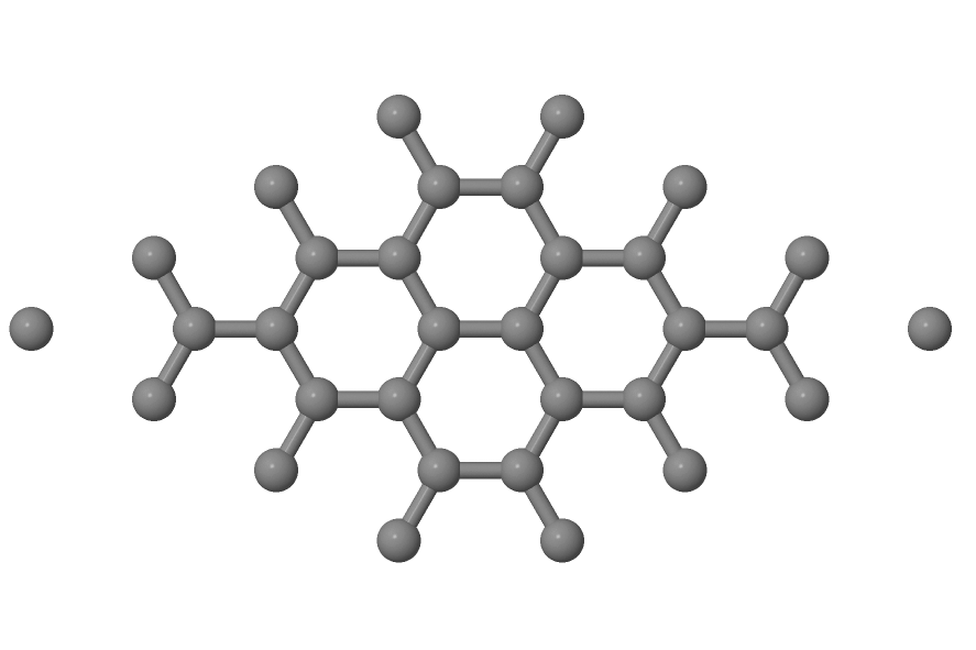
Figure 6 4x4x1 graphene supercell#
Now open the DFTB+ control file dftb_in.hsd. You should see the following options within it:
First we include the GEN-formatted geometry file, geo.gen, using the inclusion operator (
<<<):Geometry = GenFormat { <<< "geo.gen" }Then we specify the
ConjugateGradientdriver to optimize the geometry and also the lattice vectors. Since neither the angle between the lattice vectors nor their relative lengths should change during optimization, we carry out an isotropic lattice optimization:Driver = ConjugateGradient { LatticeOpt = Yes Isotropic = Yes }Then the details of the DFTB hamiltonian follow:
Hamiltonian = DFTB {Within this block, we first specify the location of the parametrization files (the Slater-Koster files) and provide additional information about the highest angular momentum for each element (this information is not yet stored in the Slater-Koster-files):
MaxAngularMomentum {
  C = "p"
}
SlaterKosterFiles = Type2FileNames {
  Prefix = "../../slako/"
  Separator = "-"
  Suffix = ".skf"
}
Please note, that the highest angular momentum is not a free parameter to be changed, but it must correspond to the value given in the documentation section of the correspoding homonuclear Slater-Koster-files (e.g. see the C-C.skf file for carbon).
We use the self-consistent charge approach (SCC-DFTB), enabling charge transfer between the atoms:
SCC = Yes
As graphene is metallic we smear the filling function to achieve better SCC-convergence:
Filling = Fermi {
  Temperature [Kelvin] = 100
}
For the Brillouin-zone sampling we set our k-points according to the 48 x 48 x 1 Monkhorst-Pack sampling scheme. This contains those k-points which would be folded onto the k-point (0.5, 0.5, 0.0) of an enlarged supercell consisting of the primitive unit cell repeated by (48, 0, 0), (0, 48, 0) and (0, 0, 1). This can be easily specified with the
SupercellFoldingoption, where one defines those supercell vectors followed by the target k-point.KPointsAndWeights = SuperCellFolding { 48 0 0 0 48 0 0 0 1 0.5 0.5 0.0 }We also want to do some additional analysis by evaluating the contributions of the s- and p-shells to the density of states (DOS). Accordingly, we instruct DFTB+ in the
Analysisblock to calculate the contribution of all C atoms to the DOS in a shell-wise manner (s and p) and store the shell-contributions in files starting with a prefix of pdos.C:Analysis { ProjectStates { Region { Atoms = C ShellResolved = Yes Label = "pdos.C" } } }
Running the code#
When you run DFTB+, you should always save its output into a file for later inspection. We suggest using a construction like this (output is saved into the file output):
dftb+ | tee output
You will see that DFTB+ optimizes the geometry of graphene by changing the lattice vectors and ion coordinates to locally minimise the total energy. As the starting geometry is quite close to the optimum one, the calculation should finish almost immediately.
Apart from the saved output file (output), you will find several other new files created by the code:
- dftb_pin.hsd
Contains the parsed user input with all the default settings for options which have not been explicitely set by the user. You should have look at it if you are unsure whether the defaults DFTB+ used for your calculation are appropriate, or if you want to know which other options you can use to adjust your calculation.
- detailed.out
Contains detailed information about the calculated physical quantities (energies, forces, charges, etc.) obtained in the last SCC cycle performed.
- band.out
Eigenvalues (in eV) and fillings for each k-point and spin channel.
- charges.bin
Charges of the atoms at the last iteration, stored in binary format. You can use this file to restart a calculation with those atomic charges.
- geo_end.xyz, geo_end.gen
Final geometry in both XYZ and GEN formats.
- pdos.C.1.out, pdos.C.2.out
Output files containing the projected density of states for the first and second angular shells of carbon (in this case the 2s and 2p shells). Their format is similar to band.out.
Analysing results#
The very first thing you should check is whether your calculation has converged at all to a relaxed geometry. The last line of the output file contains the appropriate message:
Geometry converged
This means that the program stopped because the forces on the atoms which are
allowed to move (all of them in this example) were less than a given tolerance
(specified in the option MaxForceComponent, which defaults to 1e-4 atomic
units) and not instead because the maximal number of geometry optimization steps
have been executed (option MaxSteps, default 200).
You should visualize the resulting structure using Jmol (or any other molecular visualization tool). You should probably repeat the geometry again to get a better idea how it looks like, as we did for the starting structure above. The distance between the C atoms should be very similar to those in the initial structure.
In order to visualize the density of states and the partial density of states, you should convert the corresponding human readable files (with prefix .out) to XY-format data
dp_dos band.out dos.dat
dp_dos -w pdos.C.1.out pdos.C.1.dat
dp_dos -w pdos.C.2.out pdos.C.2.dat
Please note the flag -w, which is mandatory when converting partial
density of states data for plotting. You can obtain more information about
various flags for dp_dos by issuing:
dp_dos -h
You can visualize the DOS and the PDOS for the s- and p-shells of carbon in
one picture using the plotxy tool, which is a simple command line wrapper
around the matplotlib python library (issue the command plotxy -h for
help):
plotxy --xlabel "Energy [eV]" --ylabel "DOS" dos.dat pdos.C.1.dat pdos.C.2.dat &
You can use also any other program (gnuplot, xmgrace) which can visualize XY-data. You should see something similar to Figure 7.
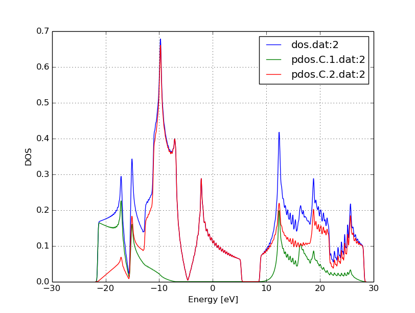
Figure 7 DOS and PDOS of graphene#
The position of the Fermi level (at -4.67 eV) can be read out from the detailed.out file, either directly or by using an appropriate grep command:
grep "Fermi level" detailed.out
As expected for graphene, the DOS vanishes at the Fermi level. Around the
Fermi level, all states are composed of the p-orbitals of the carbons, the
s-orbitals only contribute to energeticaly much lower and much higher
states. Also, one can observe the van-Hove-singularties. The wiggles at
around 0 eV and at higher energy are artifacts. Using more k-points for the
Brillouin-zone sampling or using a slightly wider broadening function in
dp_dos would smooth them out.
Band structure#
[Input: recipes/defect/carbon2d-elect/graphene/bands/]
Band structure calculations in DFTB (as in DFT) always consist of two steps:
Calculating an accurate ground state charge density by using a high quality k-point sampling.
Determining the eigenvalues at the desired k-points of the band structure, using the density obtained in the previous step. The density is not changed during this step of the band structure calculation.
Step 1 you just have executed, so you can copy the final geometry and the data file containing the converged charges from that calculation into your current working directory:
cp ../latopt/geo_end.gen .
cp ../latopt/charge.bin .
Have a look on the dftb_in.hsd file for the band structure calculation. It differs from the previous one only in a few aspects:
We use the end geometry of the previous calculation as geometry:
Geometry = GenFormat {
  <<< "geo_end.gen"
}
We need static calculation only (no atoms should be moved), therefore, no driver block has been specified.
The k-points are specified along specific high symmetry lines of the Brillouin-zone (K-Gamma-M-K):
KPointsAndWeights = KLines {
  1    0.33333333  0.66666666 0.0    # K
 20    0.0  0.0  0.0                 # Gamma
 20    0.5  0.0  0.0                 # M
 10    0.33333333  0.66666666 0.0    # K
}
We initialize the calculation with the charges stored during the previous run:
ReadInitialCharges = Yes
We do not want to change the charges during the calculation, therefore, we set the maximum number of SCC cycles to one:
MaxSCCIterations = 1
Let’s run the code and convert the band structure output to XY-format:
dftb+ | tee output
dp_bands band.out band
The dp_bands tool extracts the band structure from the file band.out and stores it in the file band_tot.dat. For spin polarized systems, the name of the output file would be different. Use:
dp_bands -h
to get help information about the arguments and the possible options for dp_bands.
In order to investigate the band structure we first look up the position of the Fermi level in the previous calculation performed with the accurate k-sampling
grep "Fermi level" ../latopt/detailed.out
which yields -4.67 eV, and then visualize the band structure by invoking
plotxy -L --xlabel "K points" --ylabel "Energy [eV]" band_tot.dat &
This results in the band structure as shown in Figure 8.
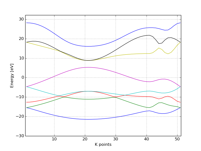
Figure 8 Band structure of graphene#
You can see the linear dispersion relations around the point K in the Brillouin-zone (k-points 0 and 51 in our circuit) which is a very typical characteristic of graphene.
Zigzag nanoribbon#
Next we will study some properties of a hydrogen saturated carbon zigzag nanoribbon.
Calculting the density and DOS#
[Input: recipes/defect/carbon2d-elect/zigzag/density/]
The initial geometry for the zigzag nanoribbon contains one chain of the structure, repeated periodically along the z-direction. The lattice vectors orthogonal to the periodicity (along the x- and y- axis) are set to be long enough to avoid any interaction between the repeated images.
First convert the GEN-file to XYZ-format and visualize it:
gen2xyz geo.gen
jmol geo.xyz &
Similar to the case of perfect graphene, you should check first the initial geometry by repeating it along the periodic axis (the third lattice vector in this example) and visualize it. The necessary steps are collected in the file checkgeo.sh. Please have a look at its content to understand what will happen, and then issue
./checkgeo.sh
to obtain the molecule shown in Figure 9.
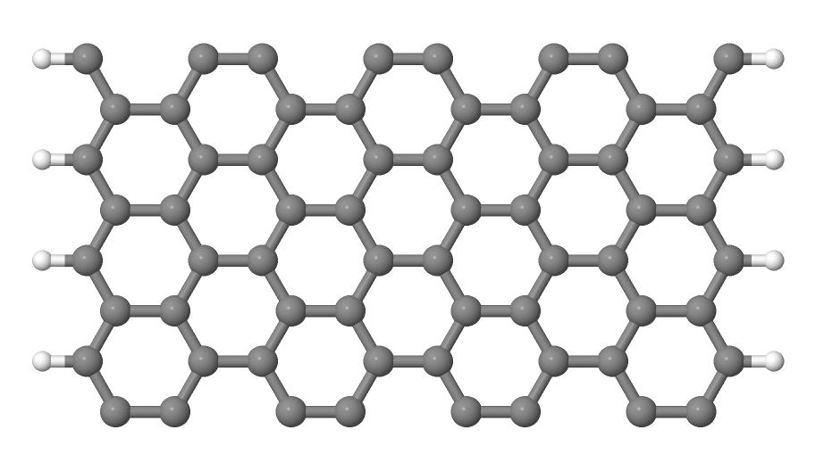
Figure 9 Section of an H-saturated zigzag nanoribbon#
The control file dftb_in.hsd is similar to the previous examples, with a few differences only:
We use the 1 x 1 x 24 Monkhorst-Pack k-point set to sample the Brillouin-zone, since the ribbon is only periodic along the direction of the third lattice vector. The two other lattice vectors have been choosen to be long enough to avoid interaction between the artificially repeated ribbons.:
KPointsAndWeights = SupercellFolding {
  1 0 0
  0 1 0
  0 0 24
  0.0 0.0 0.5
}
In order to analyze, which atoms contribute to the states around the Fermi level, we create four projection regions containing the saturating H atoms, the C atoms in the outermost layer of the ribbon, the C atoms in the second outermost layer and finally the C atoms in the third outermost layer, respectively. Since the ribbon is mirror symmetric, we include the corresponding atoms on both sides in each projection region:
ProjectStates {

  # The terminating H atoms on the ribbon edges
  Region {
    Atoms = H
    Label = "pdos.H"
  }

  # The surface C atoms
  Region {
    Atoms  = 2 17
    Label = "pdos.C1"
  }

  # The next row of C atoms further inside
  Region {
    Atoms = 3 16
    Label = "pdos.C2"
  }

  # Some more 'bulk-like' C atoms even deeper
  Region {
    Atoms = 4 15
    Label = "pdos.C3"
  }
}
You can run the program and convert the output files by issuing:
./run.sh
When the program has finished, look up the Fermi level and visualize the DOS and PDOS contributions. The necessary commands are collected in showdos.sh:
./showdos.sh
When you zoom into the area around the Fermi level (-4.57 eV), you should obtain something like Figure 10.
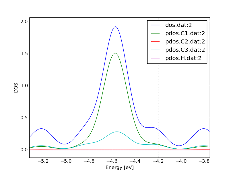
Figure 10 DOS of the zigzag nanoribbon around the Fermi energy#
You can see that the structure is clearly metallic (displaying a non-zero density of states at the Fermi energy). The states around the Fermi level are composed of the orbitals of the C atoms in the outermost and the third outermost layer of the ribbon. There is no contribution from the C atom in the layer in between or from the H atoms to the Fermi level.
Band structure#
[Input: recipes/defect/carbon2d-elect/zigzag/bands/]
Now let’s calculate the band structure of the zigzag nanoribbon. The commands are in the script run.sh, so just issue:
./run.sh
You will see DFTB+ finishing with an error message
ERROR!
-> SCC is NOT converged, maximal SCC iterations exceeded
Normally, it would mean that DFTB+ did not manage to find a self consistent charge distribution for its last geometry. In our case, however, it is not an error, but the desired behaviour. We have specified in dftb_in.hsd the options
ReadInitialCharges = Yes
MaxSCCIterations = 1
requiring the program to stop after one SCC iteration. The charges are at this point not self consistent with respect to the k-point set used for sampling the band structure calculation. However, k-points along high symmetry lines of the Brillouin-zone, as used to obtain the band structures, usually represent a poor sampling. Therefore a converged density obtained with an accurate k-sampling should be used to obtain the eigenlevels, and no self consistency is needed.
To look up the Fermi level and plot the band structure use the commands in showbands.sh:
./showbands.sh
You should obtain a band structure similar to Figure 11.
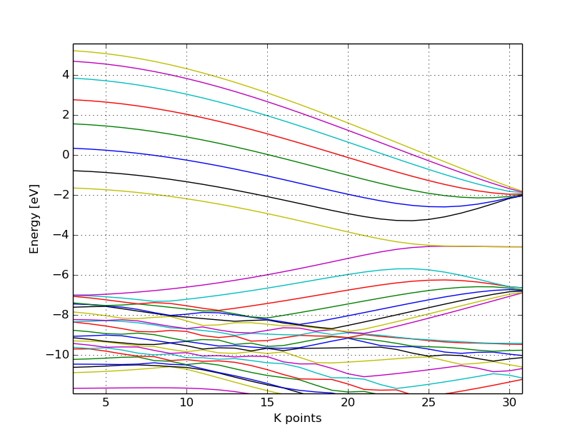
Figure 11 Band structure of the zigzag nanoribbon#
Again, one can see, that there are states around the Fermi-energy, so the nanoribbon is metallic.
Perfect armchair nanoribbon#
We now investigate a hydrogen saturated armchair carbon nanoribbon, examining both the perfect ribbon and two defective structures, each with a vacancy at a different position in the ribbon. In order to keep the tutorial short, we will not relax the vacancies, but will only remove one atom from the perfect structure.
Total energy and density of state#
[Input: recipes/defect/carbon2d-elect/armchair/perfect_density/]
The steps to calculate the DOS of the perfect H-saturated armchair nanoribbon are the same as for the zigzag case. First check the geometry with the help of repeated supercells:
./checkgeo.sh
You will see a repeated image of the perfect armchair nanoribbon unit cell (Figure 12).
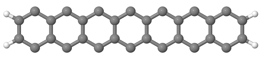
Figure 12 Perfect armchair nanoribbon unit cell#
The edge of the ribbon is visually different from the zigzag case. As it turns out, this also has some physical consequences. Let’s calculate the electronic density and extract the density of states:
./run.sh
If you look up the calculated Fermi level and then visualize the DOS
./showdos.sh
you can immediately see ( Figure 13) that there are no states around the Fermi-energy (-4.4 eV), i.e. the investigated armchair nanoribbon is non-metallic.
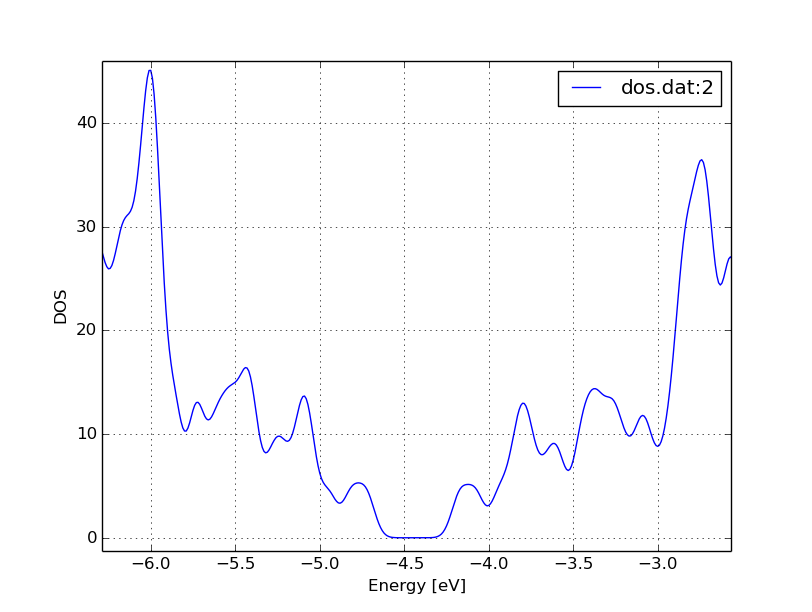
Figure 13 DOS of the perfect armchair nanoribbon#
Band structure#
[Input: recipes/defect/carbon2d-elect/armchair/perfect_bands/]
Let’s have a quick look at the band structure of the armchair H-saturated ribbon. The steps are the same as for the zigzag case, so just issue:
./run.sh
./showbands.sh
You should obtain a band structure like in Figure 14. You can read off the position of the band edges, when you zoom into the energy region around the gap: The valence band edge and the conduction band edge are in the Gamma point at -4.7 and -4.2 eV, respectively. You can also easily extract this information from the band.out file, where the occupation goes from nearly 2.0 to nearly 0.0 in the first k-point (the Gamma point).
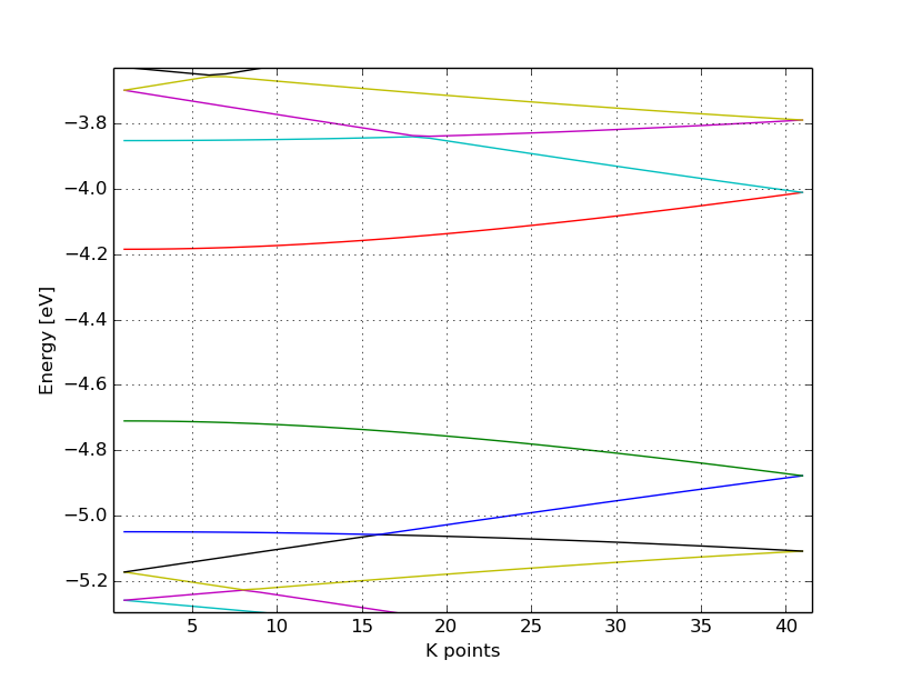
Figure 14 The band structure of the perfect hydrogen passivated armchair nanoribbon. The Fermi energy is at -4.4 eV.#
Armchair nanoribbon with vacancy#
Density and DOS#
[Input: recipes/defect/carbon2d-elect/armchair/vacancy1_density/, recipes/defect/carbon2d-elect/armchair/vacancy21_density/]
As next, we should investigate two armchair nanoribbons with a vacancy in each. The inputs can be found in the corresponding directories and you can visualize both with the command
./showgeom_v12.sh
As you can see on Figure 15 and Figure 16, the vacancy is in the two cases on different sublattices.
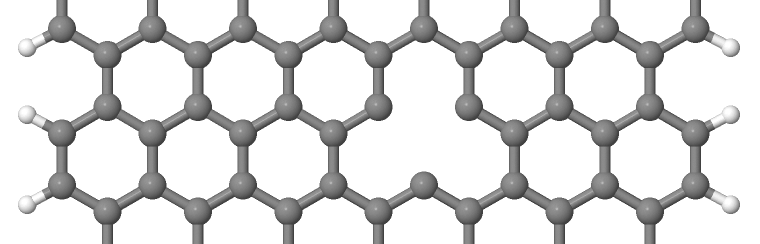
Figure 15 Armchair nanoribbon with vacancy (structure 1)#
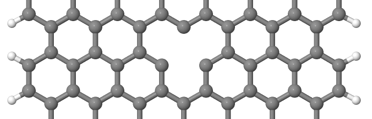
Figure 16 Armchair nanoribbon with vacancy (structure 2)#
The two vacancies (structures 1 and 2) are located on different sublattices. Since the geometries are periodic along the z-direction, the defects are also repeated. As we would like to calculate a single vacancy, we have to make our unit cell for the defect calculation large enough to avoid significant defect-defect interactions. In this case, the defective cells contain twelve unit cells.
In order to calculate the electron density of both vacancies, issue:
./run_v12.sh
This will take slightly longer than the previous calculations, since each system contains more than four hundred atoms.
We want to analyse the density of states of the two different vacancies,
together with that of the defect-free system. The commands necessary to extract
the DOS of all three configurations and show them in one figure have been stored
in the script showdos_perf_v12.sh. Execute it
./showdos_perf_v12.sh
to obtain a figure like Figure 17.
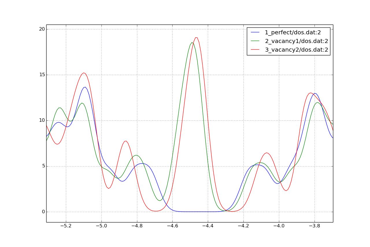
Figure 17 The DOS of the perfect nanoribbon is indicated by solid blue line, the DOS of the nanoribbons with vacancies with green and red lines, respectively.#
As you can see, in contrast to the zigzag nanoribbon, the perfect armchair nanoribbon is insulating as it has no states around the Fermi-energy (-4.45 eV). The structures with vacancies, on the other hand, introduce dangling (unsaturated) bonds, leading to unoccupied states around the Fermi-energy. We can also see, that the defects affect the band edges, which are shifted with respect to their position in the perfect structure. It also seems that the valence band edge is more affected than the conduction band edge, and in the case of vacancy 2 (red line) the effect is significantly larger than for vacancy 1 (green line).
Vacancy formation energy#
You should also be able to calculate the formation energies of the two vacancies. The formation energy \(E_{\text{form}}\) of the vacancy in our case can be calculated as
where \(E_{\text{vac}}\) is the total energy of the nanoribbon with the vacancy present, \(E_{\text{C}}\) is the energy of a C atom in its standard phase and \(E_{\text{perf}}\) is the energy of the perfect nanoribbon. Since the defective nanoribbons contain 12 unit cells of the perfect one, the energy of the perfect ribbon unit cell has to be multiplied by twelve. As a standard phase of carbon, we will take perfect graphene for simplicity. The energy of the C atom in its standard phase is then obtained by dividing the total energy of the perfect graphene primitive unit cell by two. (Look up this energy from detailed.out in the directory elect/graphene/density.) By calculating the appropriate quantities you should obtain ~8.5 eV for the formation energy of both vacancies. This is quite a high value, but you should recall that the vacancies have not been structurally optimised, and their formation energies are therefore, significantly higher than for the relaxed configurations.
Defect levels#
[Input: recipes/defect/carbon2d-elect/armchair/vacancy2_wf/]
Finally we should identify the localised defect levels for vacancy 2 and plot the corresponding one-electron wavefunctions.
The vacancy was created by removing one C atom, which had three first neighbors. Therefore, three \(\text{sp}^2\) type dangling bonds remain in the lattice, which will then form some linear combinations to produce three defect levels, which may or may not be in the band gap. The DOS you have plotted before, indicates there are indeed defect levels in the gap, but due to the smearing it is hard to say how many they are.
We want to investigate the defect levels at the Gamma point, as this is where the perfect nanoribbon has its band edges. We will therefore do a quick Gamma-point only calculation for vacancy structure 2 using the density we obtained before. We will set up the input to write out also the eigenvectors (and some additional information) so that we can plot the defect levels with waveplot later. This needs the following additional settings in dftb_in.hsd:
Options {
  WriteEigenvectors = Yes
  WriteDetailedXML = Yes
  WriteDetailedOut = No
}
To just run the calculation
./run.sh
and open the band.out file. You will see, that you have three levels (levels 742, 743 and 744 at energies of -4.51, -4.45 and -4.45 eV, respectively) which are between the energies of the band edge states of the perfect ribbon. We will visualize those three levels by using the waveplot tool.
Waveplot reads the eigenvectors produced by DFTB+ and plots real space wavefunctions and densities. The input file waveplot_in.hsd can be used to control which levels and which region waveplot should visualize, and on what kind of grid. In the current example, we will project the real part of the wavefunctions for the levels 742, 743 and 744. In order to run Waveplot, enter:
waveplot | tee output.waveplot
The calculation could again take a few minutes. At the end, you should see three files with the .cube prefix, containing the volumetric information for the three selected one-electron wavefunctions.
We will use Jmol to visualize the various wavefunction components. Unfortunately, the visualization of iso-surfaces in Jmol needs some scripting. You can find the necessary commands in the files show*.js. You can either type in these commands in the Jmol console (which should be opened via the menu File | Console…) or pass it to Jmol using the -s option at start-up. For the case latter you will find prepared commands to visualize the various orbitals in the files
./showdeflev1.sh
./showdeflev2.sh
./showdeflev3.sh
Looking at the defect levels, you can see that the defect level lowest in energy (742) has a significant contribution on the atoms around the defect, but also a non-negligible delocalized part smeared over almost all atoms in the system. Apparently a localized defect level has hybridized with the delocalized valence band edge state, resulting in a mixture between localized and non-localized state. The other two defect levels, on the other hand, have wavefunctions which are well localized on the atoms around the vacancy site. Note that in accordance with the overall symmetry of the system, the defect levels are either symmetric or antisymmetric with respect to the mirror plane in the middle of the ribbon.
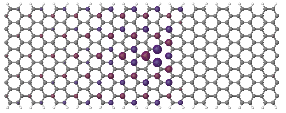
Figure 18 Wavefunction of the lowest defect level of the hydrogen saturated armchair nanoribbon with a vacancy. Blue and red surfaces indicate isosurfaces at +0.02 and -0.02 atomic units, respectively.#
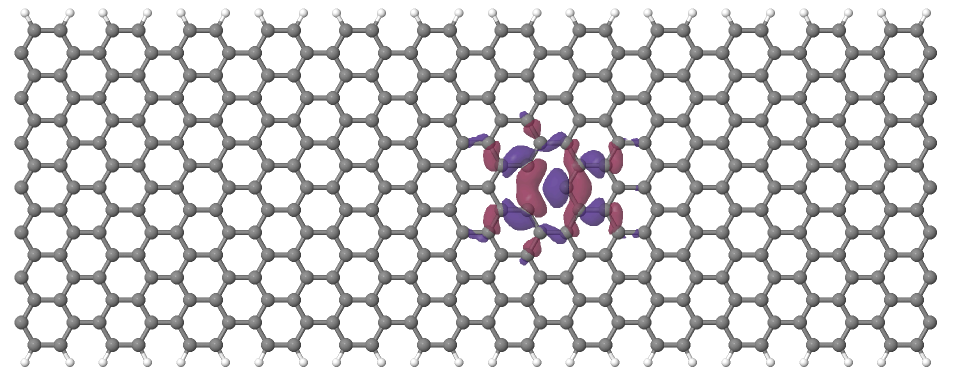
Figure 19 Wavefunction of the second lowest defect level of the hydrogen saturated armchair nanoribbon with a vacancy. Blue and red surfaces indicate isosurfaces at +0.02 and -0.02 atomic units, respectively.#
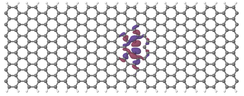
Figure 20 Wavefunction of the highest defect level of the hydrogen saturated armchair nanoribbon with a vacancy. Blue and red surfaces indicate isosurfaces at +0.02 and -0.02 atomic units, respectively.#