Example: Local Currents

[Input: recipes/transport/local-currents/]

This example guides the calculation of local atom-to-atom currents. DFTB+ can compute atom-to-atom currents starting from the general expression for the layer to layer current,

\[J = \frac{2e}{\hbar} \text{Tr} \left[H_{L,L+1} \rho_{L+1,L} - S_{L,L+1} \varepsilon_{L+1,L} - h.c. \right]\]

where \(L\) and \(L+1\) are principal layers of the transport region, \(\rho\) is the density matrix, \(\varepsilon\) is the energy-weighted density matrix, and the trace operation is used to add up all contributions. This expression is exact and guarantees current conservation along the device. From the above it is possible to write down an expression for current contributions from atom \(i\) to atom \(j\) as,

\[J_{ij} = \frac{2e}{\hbar} \sum_{\mu \in i} \sum_{\nu \in j} \text{Im} \left[ H_{\mu \nu} \rho_{\nu \mu} - S_{\mu \nu} \varepsilon_{\nu \mu}\right]\]

It should be pointed out that a derivation of the formula above is possible by, for instance, considering the time derivative of atom-projected wavefunctions but that leads to issues if the basis is not orthogonal (the DFTB case). Some implementations of local currents perform a Lowdin transformation in order to obtain orthogonalised local states to start, but we prefer to avoid such transformations that imply diagonalisation of potentially large matrices, beside the fact that with semi-infinite contacts the Lowdin rotation requires some truncation. In any case the non-locality and degree of ambiguity is not fully solved since Lowdin orbitals are quite extended.

The formulation we give still produces some issues the user should be aware of. Consider for instance a current in a linear chain with second-neighbour tight-binding interaction, as shown in Figure 51

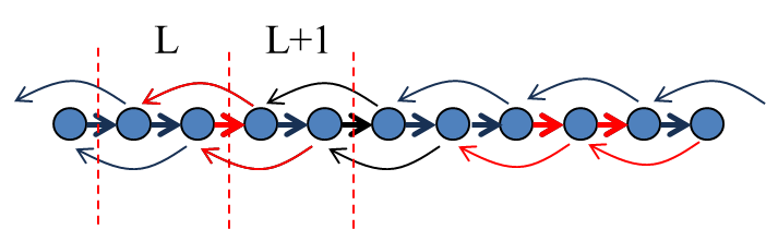
Figure 51 Bond currents in a linear chain with 2nd neighbour interactions.

Surprisingly, in the limit of low biases the bond currents between nearest neighbour atoms is positive, whereas the contribution from 2nd neighbour atoms is in the opposite direction. In units of quanta of conductance, we obtain \(J = 1.2 \text{G}_0 V\) between nearest-neighbour atoms and \(J = -0.1 \text{G}_0 V\) between second-neighbour atoms. If we cut any surface across the chain and compute the total current we correctly obtain \(J = 1.0 \text{G}_0 V\), i.e. a single quanta of conductance, as expected. The right panel of the figure above shows what happens when we compute atomic currents as a summation over bond currents. Then, for each atomic site we have an outgoing current flux of \(J = 1.2 - 0.1 = 1.1 \text{G}_0 V\). In the steady-state this is balanced by an opposite ingoing flux. Yet the net outcome of the calculation is a wrong conductance! What is missing is the 2nd neighbour contributions bypassing the next neighbour atoms. Clearly in a 1-dimensional chain this problem can be easily corrected, however in higher dimensional systems the correction might not be trivial or possible. Consider for instance the case of graphene as shown in Figure 52,

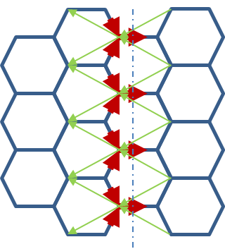
Figure 52 Bond currents in a ideal graphene with 2nd neighbour interactions.

Similar to the linear chain, the 1st neighbour currents go along the bias direction, whereas the 2nd neighbour currents point upstream. Clearly in general the contribution of 2nd or higher neighbour bond currents on each atom are not simple to include. Notice that the very same conceptual problem would occur also when the Lowdin transform is performed.

In conclusion, the local-orbital approach to bond currents produces well-defined quantities on the connection graph that however do not define a vector field. Despite this it is still useful to look at them. In the following example we show the difference between atom current and bond currents. In the second case we only consider first neighbour contributions. Atom currents on the other hand are computed as a summation of all neighbour contributions and based on the discussion above, they tend to produce a slightly overestimated result.

The reader might think that the easy solution to the problem could be to use the atomic orbitals to project the bond currents onto a real-space grid in order to recover a vector field. Unfortunately, this procedure produces strong violations of current continuity unless a complete set of orbitals is used. However the usual atomic orbital basis sets are far from complete.

Nanoribbon example

In order to obtain the local currents the user has to set the following input block:

Solver = Greensfunction {
  localCurrents = Yes
}

The reason why local currents are specified in the Greensfunction block and not within the Analysis block (e.g., TunnelingAndDos), is because the evaluation of local currents requires the Density Matrix and Energy-Weighted density matrix, according to the equations above. Hence all options concerning the contour integral apply to these calculations, rather than the options concerning the transmission function. The structure considered is shown in Figure 53.

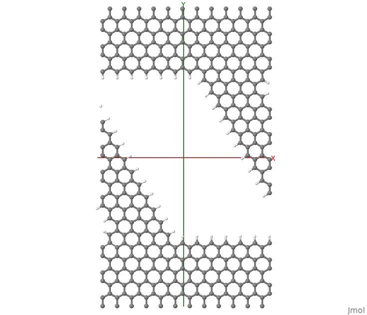
Figure 53 Nanoribbon considered in this tutorial. Periodic BC are used along X.

It consist of a nanoribbon in between graphene contacts. Periodic Boundary Conditions have been applied along the x-axis. Dangling bonds have been saturated with hydrogen atoms. In order to discuss the more complex case of currents in periodic systems, we consider a graphene nanoribbon (GNR) with a diagonal orientation. The hydrogen atoms are found very important in order to obtain a converged SCC-loop. Mulliken charges compare very well with values obtained for a supercell calculation based on usual DFTB. In order to converge the SCC loop we had to set a value for the delta-parameter in the Green’s function definition larger than the default value:

Solver = Greensfunction {
  delta = 5e-4
  localCurrents = Yes
}

This might occasionally happen when the iterative decimation solver of the surface Green’s functions fails with inversion errors or unusually long calculations that ends in NaN results. In this tutorial converged charges are precomputed and read from charges.dat. Notice that the file is stored as formatted text, hence the following option is required:

Option{
  ReadChargesAsText = Yes
}

The user might experiment restarting the SCC loop, this should take about 40 SCC iterations to converge.

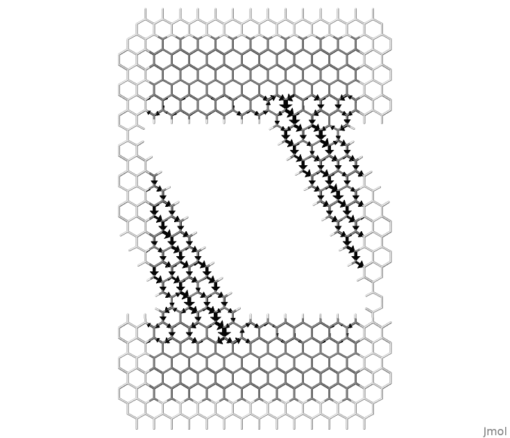
Figure 54 Local bond currents in a nanoribbon between graphene contacts.

Figure 54, shows the bond currents. This figure is obtained as a post-processing of the code outputs using the small program flux.f90, which can be found in the folder tools/misc/transport/. DFTB+ produces the following output files:

supercell.xyz
lcurrents_001_u.dat
lcurrents_u.dat

The file supercell.xyz contains the input geometry with additional atoms of the neighbour cells that are used to calculate the bond directions and draw the arrows. Notice that only bond-currents going from the central cell towards the atoms in the periodic copies are computed. The figure can be made periodic by copy-paste of repeating cells. The second file contains the k-resolved local currents, where 001 here stands for the first k-point and “u” stands for up spin. The last file contains the summation over all k-components with corresponding weights.

Make sure the program flux.f90 has been compiled and is available. The figure above was obtained by issuing the following command:

>> flux supercell.xyz -b lcurrents_u.dat 3 -w 0.3 -f 1.0 > scr.jmol

Notice the value 3 used, representing the number of neighbours considered. Then it is possible to plot this with:

>> jmol supercell.xyz -s scr.jmol

The white background colour in jmol was obtained with the jmol command:

> background white
> wireframe 0

and the black arrows can be obtained using the -c black as last option to flux.

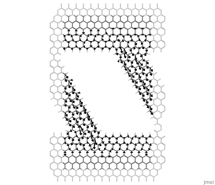
Figure 55 Local atomic currents in a nanoribbon between graphene contacts.

Similarly, it is possible to draw atomic currents shown in Figure 55, with the command:

>> flux supercell.xyz -a lcurrents_u.dat 24 -w 0.3 -f 1.0 > scr.jmol

Here we consider 24 neighbours for every atom to reach a converged result. The user can experiment by changing this value as well as well as the value used for bond currents.

The rendering of the local current as arrows in jmol is a little primitive. One difficulty is that a linear scale has a narrow window of values that can be rendered with visible arrows. Arrows representing atomic currents are adjusted in length. The option -f can be used as a global rescaling factor in order to adjust all lengths by a factor. The arrows representing bond currents are limited within the bonds. In this case, in order to emphasise different magnitudes arrow widths are used. These can be adjusted using the option -w. In most cases it might be necessary to edit flux.f90 in order to adjust the aesthetics of the rendering as desired.