Electron transport calculations in armchair nanoribbons

In this chapter we will learn how to set up self-consistent and non-self-consistent simulations with open boundary conditions by using DFTB+. We will then calculate the density of states and the transmission coefficients and analyse the results in comparison with the previous periodic calculations.

Non-SCC pristine armchair nanoribbon

[Input: recipes/transport/carbon2d-trans/agr-nonscc/ideal/]

Preparing the structure

When we run a transport calculation with open boundary conditions, the geometry specified in the input needs to obey some rules (see Specifying the geometry). The system must consist of an extended device (or molecule) region, and two or more semi-infinite bulk contacts. The bulk contacts are described by providing two principal layers for each contact.

A Principal Layer (PL) is defined as a contiguous group of atoms that have finite interaction only with atoms belonging to adjacent PLs. In a sense, a PL is a generalisation of the idea of nearest neighbour atoms to the idea of nearest neighbour blocks. The PL partitioning in the electrodes is used by the code to retrieve a description of the bulk system. PLs may be defined, as we will see, in the extended device region to take advantage of the iterative Green’s function solver algorithm.

Additional information about the definition of PLs, contacts and extended device region can be found in the manual.

In the case of an ideal one-dimensional system, all the PLs are identical. The system we start with is an infinite armchair graphene nanoribbon (AGR), therefore the partitioning into device and contact regions is somewhat arbitrary. We will therefore start from a structure file containing a single PL (2cell_7.gen), which has been previously relaxed. The PL can be converted to XYZ format by using the gen2xyz script and visualised with Jmol:

gen2xyz 2cell_7.gen
jmol 2cell_7.xyz

The structure is shown in Figure 26

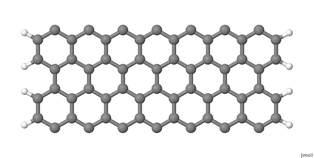
Figure 26 Armchair nanoribbon principal layer (PL)

As you may notice, we did not take a single unit cell length as a PL, but rather two unit cells of the graphene conventional unit cell. This choice is dictated by the definition of the PL itself, as we want to avoid non-zero interactions between second-neighbour PLs. This is better explained by referring to Figure Layer definition. The red carbon atoms represent the closest atoms which would belong to non-nearest neighbour PLs, and these have a separation of 0.568 nm, as shown in Figure Layer definition. The carbon-carbon interaction is non-zero up to a distance of 6 a.u., therefore the interaction between the two red atoms would be small but non-zero. Hence this is too small a separation for a one unit cell long section of nanoribbon to be used as the PL.

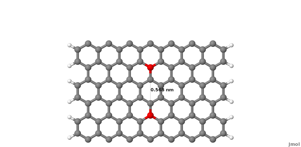
Figure 27 Layer definition

In this case the PL must contain two unit cells, in this case, as shown in figure Layer definition. It follows that the correct definition of a PL depends both on the geometry of the system and the interaction cut-off distance as defined in the SK files (In the first line of the SK-files this is given as the grid spacing in atomic units and the number of grid points in the file). The cutoff distance can be shortened slightly using the option TruncateSKRange in the Hamiltonian section, however users should be aware that this impacts the electronic properties of the system, hence should be used by experts only.

After having defined a proper PL, we then build a structure consisting of a device region with 2 PLs and contacts at each end of this region, each consisting of 2 PLs.

Note: For the pristine system, intensive properties in equilibrium calculations should not depend on the length of the device region, as the represented system is an infinite ideal nanoribbon with discrete translational symmetry along the ribbon.

The input atomic structure must be defined according to a specific ordering: the device atoms come first, then each contact is specified, starting with the PL closer to the device region. For an ideal system defined by repetition of identical PLs, the tool buildwire (distributed with the DFTB+ code) can be used to build geometries with the right ordering.

When you type:

buildwire 2cell_7.gen 3 2

the code use the geometry contained in the input supercell (2cell_7.gen), assuming direction 3 (=z) is the transport direction and that the number of principal layers in the device region will set this to be 2.

The code buildwire then will produce the correct transport block for dftb_in.hsd:

Transport{
  Device{
    AtomRange = 1 136
    FirstLayerAtoms = 1 69
  }
  Contact{
    Id = "source"
    AtomRange = 137 272
  }
  Contact{
    Id = "drain"
    AtomRange = 273 408
  }
  Task= contactHamiltonian{
    contactId = "source"
  }
}

A file Ordered_2cell_7.gen will have been created, which we will rename device_7.gen using the following:

mv Ordered_2cell_7.gen device_7.gen

We can better understand the ordering of the atomic indexes if we convert this structure to XYZ, open it with jmol and then change the colours of specific ranges of atoms by using the following syntax in the jmol console (for example, we select here the first contact and split it into two sub-ranges containing its first and second PLs):

> select atomno>136 && atomno<205
> color yellow
> select atomno>204 && atomno<273
> color red

In Figure 28 a Jmol export of the structure is shown.

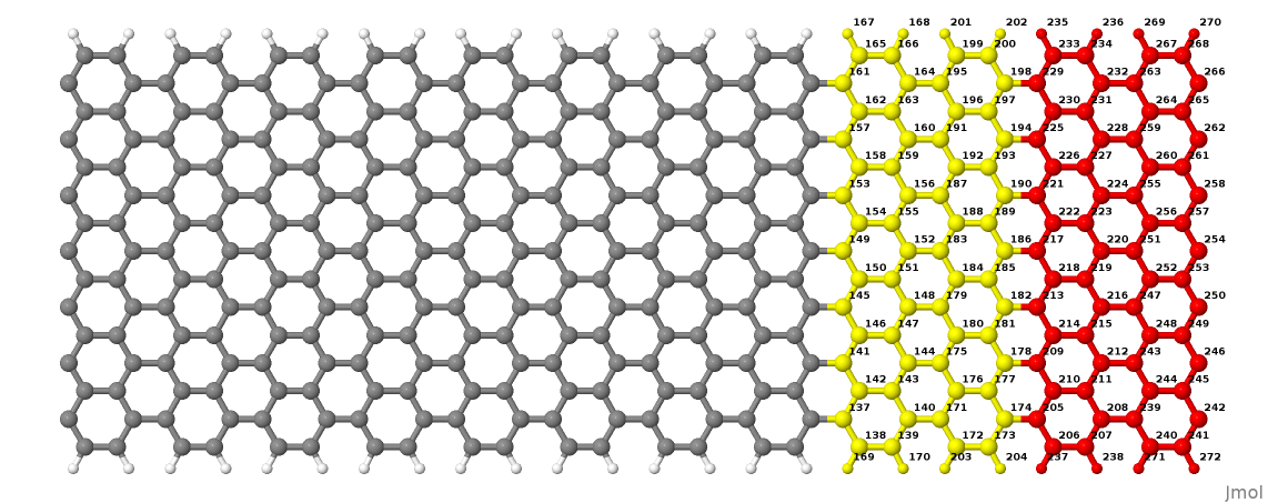
Figure 28 The PLs of contact 1

The yellow and red atoms represent the first and second PLs of the first contact. When you build a structure yourself, it is always a good idea to use a visualiser and verify that the atomic indices are consistent with the transport setup definitions.

The last step is to make sure the structure is defined as a cluster. From the point of view of an open boundary condition calculation, supercells (S) and clusters (C) have slightly different meanings compare with canonical DFTB calculations. By supercell we mean any structure which is periodic in any direction transverse to the transport direction, while for cluster we mean any structure not periodic in any direction transverse to transport. It follows that purely 1D systems, like nanowires and nanoribbons, should be regarded as clusters (C). Therefore we edit the structure file device_7.gen, changing in the first line the S (supercell) to be C (cluster) and remove the last four lines, which would normally only be defined for periodic systems. The newest versions of buildwire should automatically do this. The corrected definition for the 1D ribbon with open boundary conditions is then:

408  C
C    H
  1    1     37.831463060000    -20.000000000000      0.710000000000
  2    1     39.061219140000    -20.000000000000      1.420000000000
  3    1     39.061219140000    -20.000000000000      2.840000000000
  4    1     37.831463060000    -20.000000000000      3.550000000000
  5    1     35.371950920000    -20.000000000000      0.710000000000
  6    1     36.601706990000    -20.000000000000      1.420000000000
  7    1     36.601706990000    -20.000000000000      2.840000000000
  8    1     35.371950920000    -20.000000000000      3.550000000000
  ........
  65    2     20.880312110000    -20.000000000000    -11.870830122700
  66    2     20.880312110000    -20.000000000000     -9.429169877000
  67    2     40.025607920000    -20.000000000000    -11.870893735700
  68    2     40.025607920000    -20.000000000000     -9.429106264000

Now the file device_7.gen contains the correct structure, defined as a cluster and with the proper atom ordering. Next, we set up the input file for a tunnelling calculation.

Transmission and density of states

In the following we will first set up the simplest open boundary condition calculation: transmission coefficients according to the Landauer-Caroli formula, assuming a non-SCC DFTB hamiltonian. We will discuss and comment the different sections contained in the file dftb_in.hsd.

First, we have the specification of the geometry:

Geometry = GenFormat {
<<< 'device_7.gen'
}

This follows the same rule as in a regular DFTB+ calculation, except for the fact that the structure should follow the specific partitioning structure explained in the previous section.

Whenever an open boundary system is defined, we have to specify a block named Transport which contains information on the system partitioning and additional information about the contacts to the device:

Transport {
  Device {
    AtomRange = 1 136
    FirstLayerAtoms =  1 69
  }
  Contact {
    Id = "source"
    AtomRange = 137 272
    FermiLevel [eV] = -4.7103
    potential [eV] = 0.0
  }
  Contact {
    Id = "drain"
    AtomRange = 273 408
    FermiLevel [eV] = -4.7103
    potential [eV] = 0.0
  }
}

Here we have used the indexes printed by buildwire. Device contains two fields: AtomRange specifies which atoms belong to the extended device region (1 to 136) and FirstLayerAtoms specify the starting index of the PLs in the device region. This field is optional, but if not specified the iterative algorithm will not be applied and the calculation will be slower, even though the result will be still correct. Then we have the definitions of the contacts. In this example we define a two terminal system, but in general N contacts are allowed. A contact is defined by an Id (mandatory), the range of atoms belonging to the contact specified in AtomRange (mandatory) and a FermiLevel (mandatory). The potential is set by default to 0.0, therefore need not be specified in this example.

Note that in non-SCC calculations that do not compute the Density Matrix of the system, the Fermi level and the contact potential are not necessary to calculate a transmission curve, but they are needed to calculate the current via the Landauer formula, as they would determine the occupation distribution in the contacts.

Then we have the Hamiltonian block, describing how the initial Hamiltonian and the SCC component, if any, will be calculated:

Hamiltonian = DFTB {
  SCC = No
  MaxAngularMomentum {
    C = "p"
    H = "s"
  }
  SlaterKosterFiles = Type2FileNames {
    Prefix = "../../slako/"
    Separator = "-"
    Suffix = ".skf"
  }
  Solver = TransportOnly{}
}

In this example we will calculate the transmission according to the Caroli (referred by some authors as the Fisher Lee) formula in a non-SCC approximation, i.e. the Hamiltonian is directly assembled from the Slater-Koster files and used “as is” to build the contact self energies and the extended device Green function. The use of an eigensolver is not meaningful in an open boundary setup, as the system is instead solved by the Green function technique. Therefore we just use a keyword TransportOnly to indicate that we do not want to solve an eigenvalue problem. The other fields are filled up in the same way as for a regular DFTB calculation.

Usually in DFTB+ an eigensolver is regarded as a calculator which can provide the charge density in the SCC cycle, therefore we will instead define a Green’s function based solver later, but only for SCC calculations.

Note that as C-H bonds are present in the system, charge transfer should occur, hence the result will not be accurate at the non-SCC level. It is not a-priori trivial to predict whether this affects qualitatively or quantitatively the transmission. We will therefore later compare these results with an SCC calculation - at the moment we will stay at the level of a non-SCC calculation, because it is faster to execute and also allows us to use the simplest input file possible.

Finally, the implementation of the Landauer-Caroli formula is regarded as a post-processing operation and specified by the block TunnelingAndDos inside Analysis:

Analysis {
  TunnelingAndDos {
    Verbosity = 101
    EnergyRange [eV] = -6.5  -3.0
    EnergyStep [eV] = 0.01
    Region {
      Atoms = 1:136
    }
  }
}

TunnelingAndDos allows for the calculation of Transmission coefficient, Local Density of States (LDOS) and current. A transmission is always calculated using the energy interval and energy step specified here. The LDOS is only calculated when sub-blocks Region are defined. Region can be used to select some specific subsets of atoms or orbitals, according to the syntax explained in the manual. In this example, we are specifying the whole extended device region (atoms 1 to 136). Note that the energy range of interest is not known a-priori. Either you have a reference band structure calculation so therefore know where the first sub-bands are (the correct way to do this), or you can run a quick calculation with a large energy step and on the basis of the transmission curve then refine the range of interest.

We can then start the calculation:

dftb+ dftb_in.hsd | tee output.log

Parallelism in transport calculations

Please have have a look at the section Parallel usage of DFTB+ for a general discussion. In transport calculations we can take advantage of parallelisation over the energy points by running the (mpi enabled) code with mpirun:

mpirun -n 4 dftb+ dftb_in.hsd | tee output.log

where 4 should be substituted by the number of available nodes. Note that non-equilibrium Green’s function (NEGF) calculations are parallelised over energy points, therefore a number of nodes larger than the energy grid will not improve performances and secondly that the memory consumption is proportional to the number of nodes used - this may be critical in shared memory systems with a small amount of memory per node. SMP parallelism is also used via OpenMP multi-threading, this is exploited at low level linear algebra numerics such as Matrix-Matrix multiplications and Matrix inversions, especially when linking to libraries such as the Intel MKL. Multi-threading is not enabled by default in DFTB+ since this can easily collide with the parallel SCALAPACK diagonaliser. In order to enable OMP calculations you should explicitly look for Parallel block:

Parallel{
  UseOmpThreads = Yes
}

Some experimentation can be done in order to find the optimal combination of MPI and OpenMP. Clearly the two schemes should not overlap on the same CPU(s). For instance in the early days Xeon Quad Cores CPUs the best performances could be obtained by running OpenMP with maximum of 4 threads (OMP_NUM_THREADS=4) and MPI across as many separate nodes or sockets as available. As the number of cores on each socket has increased to 8, 10 or more, the most efficient balance has to be determined by testing. Typically openMP does not scale quite linearly but tend to saturate at about 4 threads for typical transport calculations. Therefore it seems optimal to divide the total number of available cores modulo 4 threads to get the number of MPI processes. So, for instance with 64 cores spread on 4 units with 2 sockets of 8 cores each, it should be fine to set OMP_NUM_THREADS=4 and 16 MPI processes.

Plotting Transmission and DOS

When the calculation has finished, the transmission and density of states are saved to separate transmission.dat and localDOS.dat files. These additional files both contain the energy points in the first column and the desired quantities as additional columns.

We can plot the transmission by using the plotxy script:

plotxy --xlabel 'Energy [eV]' --ylabel 'Transmission' -L transmission.dat

The plot is shown in Figure 29:

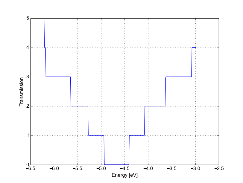
Figure 29 Non-SCC transmission through a pristine AGR

The ribbon is semiconducting, therefore we can see a zero transmission at energies corresponding to the band gap. As the system is ideal, outside of the band gap we can observe the characteristic conductance steps where the value of the transmission is 1.0 for every band which crosses a given energy. This is a normal signature of ideal 1D systems with translational invariance.

Similarly, we can visualise the density of states by typing (the x and y axis limits are chosen to focus on the first few sub-bands):

plotxy --xlabel 'Energy [eV]' --ylabel 'DOS [arbitrary units]' -L \
--xlimits -6.5 -3 --ylimit 0 1400 localDOS.dat

The result is shown in Figure 30:

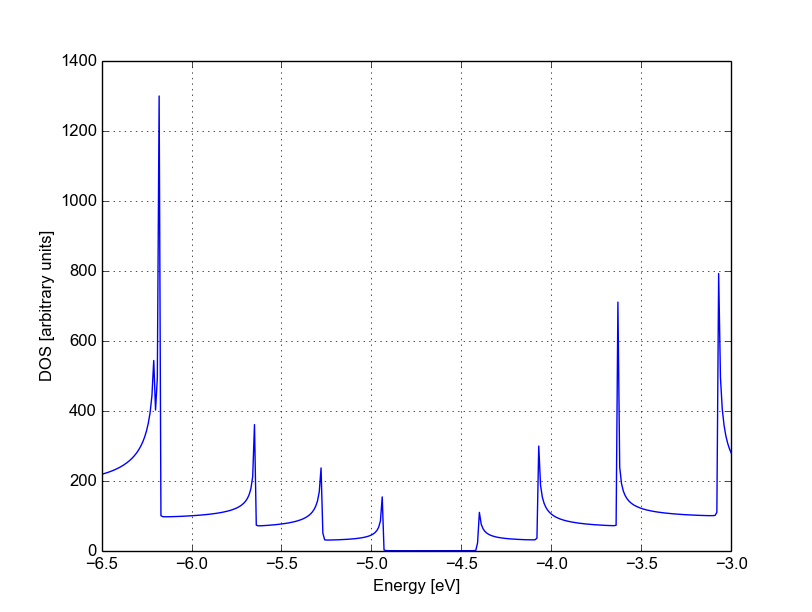
Figure 30 Non-SCC density of states for a pristine AGR

You can plot the transmission or the density of states on a semi-logarithmic scale:

plotxy --xlabel 'Energy [eV]' --ylabel 'Transmission' -L \
--xlimits -6.5 -3 --logscale y localDOS.dat

If you do so, you will obtain the plot shown in Figure Non-SCC density of states on logarithmic scale.

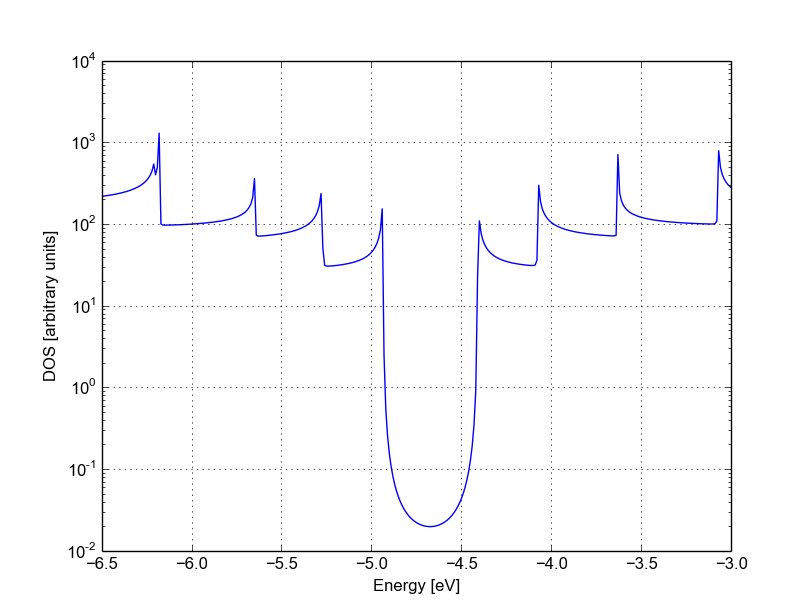
Figure 31 Non-SCC density of states on logarithmic scale

The density of states inside the band-gap is not zero, but decreases by several orders of magnitude. This is a natural consequence of the quasi-particle nature of the Green’s function formalism: every state in the system has a finite broadening in energy.

Non-SCC armchair nanoribbon with vacancy (A)

[Input: recipes/transport/carbon2d-trans/agr-nonscc/vacancy1/]

Transmission and Density of States

Now that we have a calculation of the reference pristine system, we will introduce a scattering centre by producing a vacancy in the system. In order to do so, we directly modify the structure file device_7.gen and the input file dftb_in.hsd. We remove atom number 48 from the structure file. Note that DFTB+ ignores the indexes in the first column of the .gen file, therefore we do not need to adjust them. We have, however, to remember to change the total number of atoms in the first line from 408 to 407:

407  C
C    H
1    1     37.831463060000    -20.000000000000      0.710000000000
2    1     39.061219140000    -20.000000000000      1.420000000000
3    1     39.061219140000    -20.000000000000      2.840000000000
.....
46    1     32.912438770000    -20.000000000000      7.810000000000
47    1     30.452926620000    -20.000000000000      4.970000000000
49    1     31.682682700000    -20.000000000000      7.100000000000
50    1     30.452926620000    -20.000000000000      7.810000000000
...

The resulting structure should look like this:

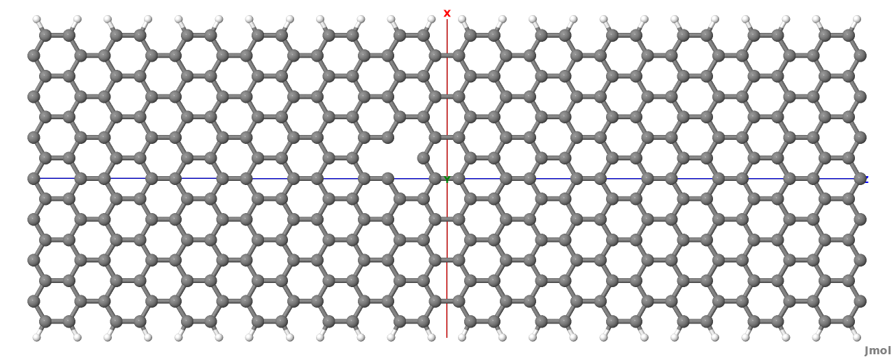
Figure 32 Geometry with vacancy on sublattice A

We then also adjust the dftb_in.hsd file accordingly. As we have removed an atom, all the indexes in the transport block need to be adjusted properly. Note that we removed an atom in the first PL of the extended device, therefore we also need to adjust the values of FirstLayerAtoms. The Transport block now reads:

Transport {
    Device {
      AtomRange = 1 135
      FirstLayerAtoms =  1 68
    }
    Contact {
      Id = "source"
      AtomRange = 136 271
      FermiLevel [eV] = -4.7103
      potential [eV] = 0.0
    }
    Contact {
      Id = "drain"
      AtomRange = 272 407
      FermiLevel [eV] = -4.7103
      potential [eV] = 0.0
    }
}

Compared to the pristine system, we have modified AtomRange in all the blocks and the values of FirstLayerAtoms.

After running the calculation, we can compare the transmission curve for this structure with a single vacancy and the pristine ribbon by using plotxy:

plotxy --xlabel 'Energy [eV]' --ylabel 'Transmission' -L --xlimits -6.5 -3 \
transmission.dat ../ideal/transmission.dat

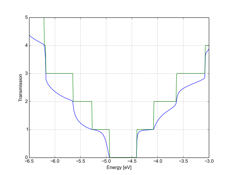
Figure 33 Non-SCC Transmission in pristine (green) and single vacancy (blue) ribbons

Clearly, the presence of a vacancy introduces some finite scattering which reduce the transmission with respect to the ideal ribbon. In particular, the effect is quite small in the first conductance band while it is more visible in the first valence band and in higher bands. The reflection amplitude is increased near the band edges. This is expected in 1D systems, as near the band edges the density of states diverges (Van Hove singularities), hence the group velocity is lower, and it is known from semi-classical transport theory that the scattering probability is, when short range disorder is present, inversely proportional to the group velocity. The absence of resonant features in the transmission may point to the fact that the vacancy does not induce additional states in the conduction or valence bands. This can be verified by visualising the density of states, as in Figure Non-SCC DOS for single vacancy in sublattice A (linear scale).

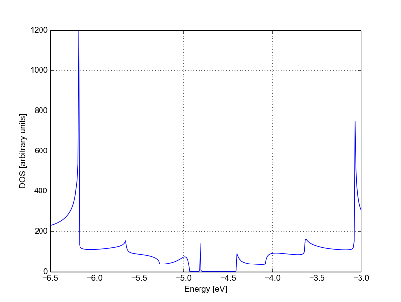
Figure 34 Non-SCC DOS for single vacancy in sublattice A (linear scale)

The same density of states can be visualised on logarithmic scale as well, as in Figure 35.

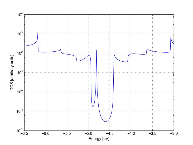
Figure 35 Non-SCC DOS for single vacancy on sublattice A (semilog scale)

The vacancy is adding some close energy levels in the gap, as verified already using a conventional DFTB+ calculation (Armchair nanoribbon with vacancy). The Van Hove singularities are partially suppressed as the system no longer possesses translational symmetry along the transport direction. Even in a simple non-SCC approximation, the qualitative picture is consistent with the previous SCC periodic calculation. We will now consider a vacancy sitting on the other sublattice (B) and try to understand whether the relative position of the vacancy is relevant or not by calculating once more the non-SCC transmission and density of states.

Non-SCC armchair nanoribbon with vacancy (B)

[Input: recipes/transport/carbon2d-trans/agr-nonscc/vacancy2/]

Transmission and Density of States

We will now consider a vacancy sitting on the other sublattice (B), i.e. we can take the structure file we used for the ideal ribbon and instead delete the atom number 47. The structure file is:

407  C
C    H
1    1     37.831463060000    -20.000000000000      0.710000000000
2    1     39.061219140000    -20.000000000000      1.420000000000
3    1     39.061219140000    -20.000000000000      2.840000000000
.....
46    1     32.912438770000    -20.000000000000      7.810000000000
48    1     31.682682700000    -20.000000000000      5.680000000000
49    1     31.682682700000    -20.000000000000      7.100000000000
50    1     30.452926620000    -20.000000000000      7.810000000000
.....

The jmol rendering of the geometry:

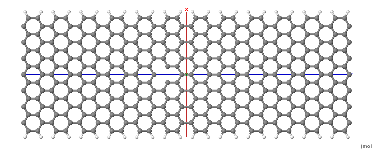
Figure 36 Geometry with vacancy on sublattice B

Also in this case we remove an atom from the first PL of the extended device region, therefore the rest of the dftb_in.hsd input file is identical to the one we used for the vacancy on sublattice A. We can therefore just copy it and run the DFTB calculation. The transmission is shown in Figure Non-SCC Transmission for vacancy B (blue), pristine (green) and vacancy A (green) (transmission for vacancy on sublattice B in blue, transmission for vacancy on sublattice A in green and pristine system in green):

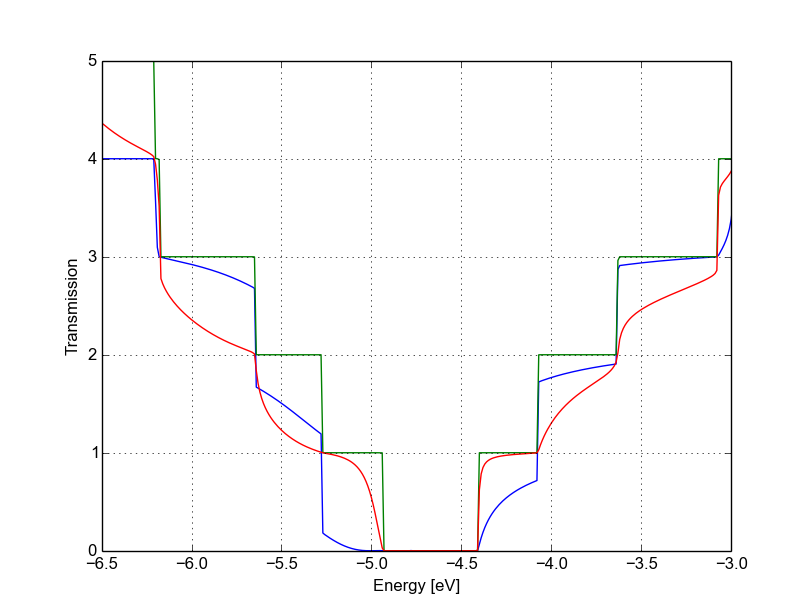
Figure 37 Non-SCC Transmission for vacancy B (blue), pristine (green) and vacancy A (green)

We can see a very strong suppression of transmission in the first sub-bands, especially in the first valence band. Again, the absence of resonances may be due by gap states. In fact, we can verify it by plotting the density of states, as shown in Figure 38.

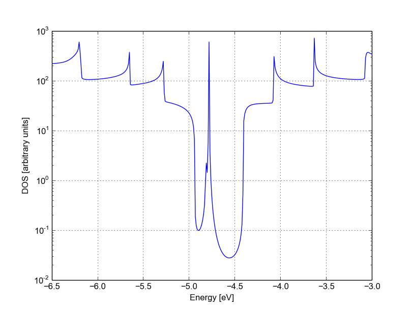
Figure 38 Non-SCC DOS for vacancy in sublattice B

We can clearly see that the vacancy induces some nearly degenerate gap states, and that the density of states at higher energies is largely unaffected. It is known that the relative position of a scattering centre in a graphene nanoribbon with respect to different sub-lattices strongly affects its transport properties, as is shown in these non-SCC calculation. Qualitatively, the picture is also consistent with periodic DFTB+ calculations, with the difference that we directly obtain information on the effect on transport properties via transmission function. This also ensures that we do not have to worry about choosing the right supercell or k-point sampling as the open boundary conditions represent exactly the infinite system with a single scattering centre. As already pointed out earlier, there is no warranty that a non-SCC calculation will give the proper result in a system if relevant charge transfer is occurring, and in general it will not. Therefore in the next section we will repeat the same calculation by solving the SCC problem.

SCC Pristine armchair nanoribbon

A DFTB Hamiltonian is in general given by two terms:

\[H^{SCC} = H^{0} + H^{\text{shift}}\]

Where the component \(H^{\text{shift}}\) is the self-consistent (SCC) correction. The SCC correction is in general needed whenever there is a finite charge transfer between atoms, i.e. whenever there are bonds between atoms with different chemical species or with different coordination numbers. In our case, we can expect a finite charge transfer between the C and H atoms at the edges, and an SCC component may be relevant due to this charge transfer. While in the previous sections, we have only considered the non-SCC component \(H^{0}\), in the next sections we will compute the same calculation by including the correction given by the shifts \(H^{\text{shift}}\).

Note that the equilibrium SCC problem can be tackled in two ways: we could apply the Landauer-Caroli to an SCC Hamiltonian taken, for example, from a periodic calculation (i.e. uploading the SCC component), or we can solve the problem as a full NEGF setup with 0 bias. The code flow is currently such that this second procedure has to be used (however, the first technique will be available in future release). Therefore we will need to learn to set up the input related to two other components of the NEGF machinery: the real space Poisson solver and the Green’s function solution of the density matrix.

In this way we will introduce a first complete input file. It is important, from a didactic point of view, to be clear that as long as the applied bias is zero and we are interested in equilibrium properties, the two approaches are equivalent and the results are only valid in the limit of linear response.

Contact calculation

[Input: recipes/transport/carbon2d-trans/agr-scc/contacts/]

In order to run an SCC transport calculation, the code needs some additional knowledge about the contact PLs. In particular, the SCC shifts and Mulliken charges have to be saved somewhere to enable consistency between the calculation of the self-energy and the calculation of the Poisson potential. To this end, we have to introduce an additional step in the procedure: the contact calculation.

The contact calculation is simply a periodic calculation for the contact PL. As such, not all the field defined in the transport are meaningful and the input file will of course look different. The Geometry block is identical:

Geometry = GenFormat {
<<< 'device_7.gen'
}

While the Transport block needs to be modified as follows:

Transport {
    Device {
      AtomRange = 1 136
    }
    Contact {
      Id = "source"
      AtomRange = 137 272
    }
    Contact {
      Id = "drain"
      AtomRange = 273 408
    }
  Task = ContactHamiltonian {
     ContactId = "source"
  }
}

We first notice the addition of an option Task =ContactHamiltonian {...}, which was previously absent. This block specifies that we intend to calculate the bulk contact SCC properties, and the field ContactId specifies which contact we want to calculate. The field FirstLayerAtoms in the Device block is absent (it does not make sense in a contact calculation) and so are the fields FermiLevel and Potential in the two Contact sections, as they are not meaningful during this step. In general, the philosophy of a DFTB+ input file is that if input fields that would be useless or contradictory are present, the code will halt with an error message.

The Hamiltonian block shows some differences, too:

Hamiltonian = DFTB {
  SCC = Yes
  SCCTolerance = 1e-6
  EwaldParameter = 0.1
  MaxAngularMomentum {
    C = "p"
    H = "s"
  }

  SlaterKosterFiles = Type2FileNames {
    Prefix = "../../slako/"
    Separator = "-"
    Suffix = ".skf"
  }

  KPointsAndWeights = SupercellFolding {
    25 0 0
    0 1 0
    0 0 1
    0.0 0.0 0.0
  }
}

The flags SCC = Yes and SCCTolerance = 1e-6 enable the SCC calculation. A tight tolerance in the contact calculation, and in general in transport calculations, helps to avoid artificial mismatches at device/contact boundaries. The other parameters are the usual ones, except for the KPointsAndWeights, which deserves special attention.

The bulk contact is of course a periodic structure, hence we need to specify a proper k-point sampling, as we would do in a regular periodic DFTB calculation. However, you should be careful about the way the lattice vector is internally defined. When the input system is a cluster (C), i.e. it has no periodicity in directions transverse to the transport direction(s), the lattice vector of the contact is internally reconstructed and assigned to be the first lattice vector, regardless the spatial orientation of the structure. This means that the KPointsAndWeights for a cluster system are always defined as above: a finite number of k-points along the first reciprocal vector (according to a 1D Monkhorst-Pack scheme) and sampling with values of 0 along the other two directions. The reason for this choice is that we do not want to assign a specific direction to the structures, i.e. at this level we do not assume in any way that the structure must be oriented along x,y or z direction.

Note also that as the contact information is used in the transport calculation, it is a good idea to use a dense k point sampling and a low SCC tolerance, in order to get a very well converged solution. The contact calculation will be usually much faster than the transport calculation, so this does not usually present a problem.

On the other hand, this rule regarding k-points does not apply to periodic transport calculations, as the periodicity along the transverse directions must also be preserved (refer to the following section for a periodic system example). We can run the calculation by typing:

dftb+ dftb_in.hsd | tee output.log

After running the calculation, we notice that a file shiftcont_source.dat is generated. This file contains the information useful for the transport calculation (shifts and charges of a bulk contact). It is suggested you also keep a copy of the detailed.out for later reference. We can obtain the value of the Fermi energy, which we will later need, from detailed.out as -4.7103 eV (this is also stored in the “shiftcont_*.dat” files).

We can now run the same calculation for the drain contact by just modifying the Task block:

Task = ContactHamiltonian {
     ContactId = "drain"
  }

The contact are identical, therefore we expect the same results, also with the same Fermi energy. We now have a file shiftcont_drain.out, which is equivalent to shiftcont_drain.dat apart from small numerical error. In fact, we could have simply copied the previous contact results into this file.

Now that the contact calculation is available, we can set up the transport calculation.

Transmission and Density of States

[Input: recipes/transport/carbon2d-trans/agr-scc/ideal/]

In order to calculate the transmission for the SCC system, we have to copy the files shiftcont_drain.dat and shiftcont_source.dat into the current directory:

cp ../contacts/shiftcont* .

Then we have to specify some additional blocks with respect to a non-SCC transport calculation. We first look at the Transport block itself:

Transport {
  Device {
    AtomRange = 1 136
    FirstLayerAtoms =  1 69
  }
  Contact {
    Id = "source"
    AtomRange = 137 272
    FermiLevel [eV] = -4.45
    potential [eV] = 0.0
  }
  Contact {
    Id = "drain"
    AtomRange = 273 408
    FermiLevel [eV] = -4.45
    potential [eV] = 0.0
  }
  Task = UploadContacts {
  }
}

The atom indices are of course the same, as the geometry of the system is not changed. This time though, we explicitly specified a Task block named UploadContacts, which declares that we are now running a full transport calculation. Task = UploadContacts {} is the default and does not take any additional parameters, therefore you can safely omit it.

Now that we are solving the full SCC scheme, we will allow for charge transfer between the open leads and the extended device region, therefore it is important to set a well-defined Fermi energy. While this does not make any difference in a non-SCC transmission calculation, it is crucial for the SCC calculation. A wrong or unphysical Fermi energy will lead to incorrect charge accumulation or depletion of the system.

To this end, you will have to pay some attention to the definition of the Fermi energy. As we are calculating a semiconductor system, the Fermi level should be in the energy gap. By calculating a band structure or by inspection of the eigenvalues in the file detailed.out you can verify that the value -4.7103 is on the edge of the valence band. This can be explained as numerically the Fermi level is defined by filling the single particle states till the reference density is reached. Its position inside the gap of a semiconductor is in some senses arbitrary within that range (a common convention which DFTB+ uses is to set it at the middle of the gap). Therefore, while in metallic system we may ensure consistency and use a well converged Fermi level at some specific temperature during all our transport calculation, in the case of a semiconductor system we can manually set the Fermi level in the middle of the energy gap (for this system, roughly at -4.45 eV) and freely vary the temperature as long as the gap is larger than several times the value of kT.

We will see in the following that there are some ways to verify that the Fermi level is defined consistently, as this is often source of confusion. Note also that, differently from other codes, DFTB+ allows for different Fermi levels in different contacts, which can be useful when heterogeneous contacts are defined (for example, in a PN junction). In that case a built-in potential is internally added to ensure no current flow at equilibrium.

In the Hamiltonian block now an SCC calculation has to be specified:

Hamiltonian = DFTB {
  SCC = Yes
  SCCTolerance = 1e-6
  ReadInitialCharges = No
  ...

Poisson Solver

Differently from the non-SCC calculation, we now need to specify a way to solve the Hartree potential and the charge density self-consistently. In a NEGF calculation, we use a real-space Poisson solver to calculate the potential, and a Green function integration method to calculate the density matrix:

...
Electrostatics = Poisson {
  PoissonBox [Angstrom] = 40.0 30.0 30.0
  MinimalGrid [Angstrom] = 0.5 0.5 0.5
  SavePotential = Yes
}

The Poisson section contains the definition of the real space grid parameters. Note that differently from a normal DFTB+ calculation, simulating regions of vacuum is not for free, as the simulation domain must be spanned by the real space grid. The grid is always oriented along the orthogonal cartesian coordinate system. PoissonBox specifies the lateral length of the grid. The length along the transport direction is ignored as it is automatically determined by the code (in this case, z=30.0). The length along the transverse direction are relevant and should be carefully set. In order not to force unphysical boundary conditions, you may extend the grid at least 1 nm away. If a strong charge transfer is present, you may go for a larger box, according to your available computational resources. A poorly defined grid can lead to no convergence at all, to a very strange (and slow) convergence path or to unphysical results. MinimalGrid specifies the minimum step size for the multigrid algorithm. Values between 0.2 and 0.5 are usually good, where a lower value stands for higher precision. SavePotential = Yes will return a file containing the potential and charge density profile, for later reference. These files can be quite large, therefore the default is No.

Density Matrix Calculations - GreensFunction solver

The solver is now specified as GreensFunction. With this definition, we instruct the code not to solve an eigenvalue problem but rather to calculate the density matrix by integration of the Keldysh Green function:

Solver = GreensFunction{}

This block provides the SCC charge density with or without applied bias. The options define the integration path. Usually the default options are good enough in most cases and advanced users may refer to the manual or other examples in this book.

The Mixer options is present in DFTB+ calculations as well.:

Mixer = Broyden {
  MixingParameter = 0.02
}

Convergence is known to be critical in NEGF schemes. In that case, a low MixingParameter value will help to avoid strong oscillation in the SCC iterations.

The last block is Analysis:

Analysis {
  TunnelingAndDos {
    Verbosity = 101
    EnergyRange [eV] = -6.0  -3.0
    EnergyStep [eV] = 0.01
  }
}

This block is identical to the non-SCC calculation as the same task is performed: calculation of Transmission, current and DOS by using the Landauer-Caroli formula. The Transmission will be of course be different due to the fact that the ground state charge density is now solution of the SCC Hamiltonian and we have slightly changed the energy range as the SCC component introduce a shift of the band-structure (try to compare the SCC and non-SCC transmission results when you are done). We can now run the calculation:

mpirun -n 4 dftb dftb_in.hsd | tee output.log

Where -n 4 should be adapted to the number of available nodes. As transport calculations in DFTB+ are parallelised on energy points, a quantity larger than 40 (the default number of integration points at equilibrium) will not speed up the calculation of the density matrix.

An inspection of the file detailed.out reveals that we have additional information with respect to the non-SCC calculation, including a list of atomic charges and orbital population, as now the SCC density matrix has been calculated. The transmission is also saved as separate file, and is shown in Figure 39.

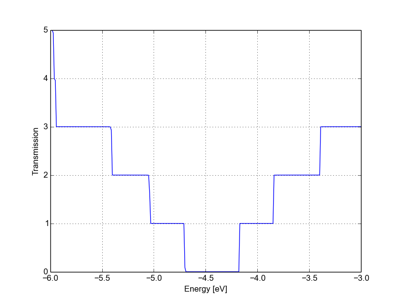
Figure 39 SCC transmission in pristine AGR

As you would expect, it still step-like as in the non-SCC calculation. This is correct, as we’re calculating an ideal 1D system. The bandwidth (i.e., the steps width) may differ due to SCC contribution and the overall transmission is shifted. Note that while the non-SCC calculation is very robust, meaning that you will always get step-like transmission for a 1D system, in the SCC calculation a poor definition of the boundary conditions, of the bulk contact properties or of the additional GreensFunction and Poisson blocks may induce numerical artefacts and scattering barriers which should not be there. As a result, the transmission will not appear step-like but rather visibly smoothed out.

You can also verify the quality of the calculation by inspection of the potential and charge density profiles. In a pristine periodic system we would expect a periodic potential, without discontinuities at the boundary between extended device and electrodes. The information needed to construct the real space potential and charge density are contained in 5 files: box3d.dat, Xvector.dat, Yvector,dat, Zvector.dat, potential.dat and charge_density.dat. The first 4 files contain the grid information, and the last two ones the list of potential and charge density values (following a row major order). Those information can be converted to any useful with some simple scripting, we provide an utility called makecube which can be used to convert them to Gaussian cube format or a more flexible vtk format. There’s plenty of software to visualise vtk or cube files, but unluckily at present current choices of software which are effective at visualising real space grid data are weak at visualising atomistic structures, and vice versa. In the following we will use paraview and work with the vtk format. Paraview is freely available and is supplied with many gnu/linux distributions as a compiled package.

The vtk file can be obtained by simply running:

makecube potential.dat pot.vtk

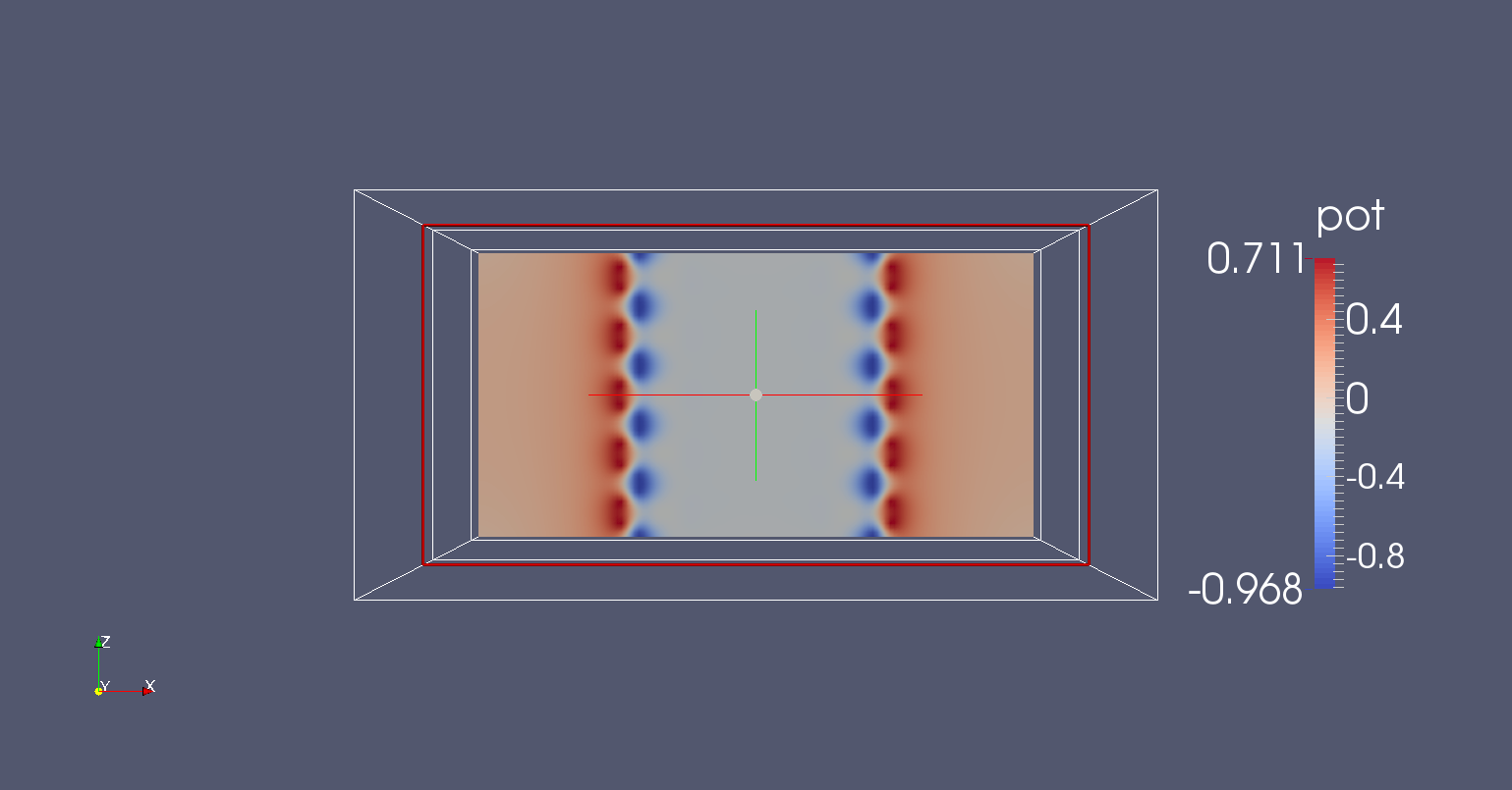
Figure 40 Potential profile along the nanoribbon

An extensive explanation of paraview features is beyond the scope of this tutorial. Following some easy steps, you can produce the potential map shown in Figure 40.

1. Open paraview and import the file pot.vtk from File->Open
2. Click on Properties->Apply (Properties are usually visualised on the left side of the screen) and you should see the bounding box in the visualisation windows.
3. In the Pipeline browser select the file pot.vtk by clicking once on it, and then select the Clip filter from Filters->Alphabetical (or from the filter toolbar).
4. In Properties, click on ‘Y Normal’ to produce a clip along the nanoribbon.
5. Click on Properties->Apply.

The plot shown in Figure 40 above is the self-consistent potential along the nanoribbon. We can see that the charge transfer between carbon and hydrogen at the edges results in a non-flat potential. At a first glance, the potential looks quite homogeneous, meaning that there are no clear discontinuities at the box boundary. This is important: being it a homogeneous ribbon, the potential should have the same periodicity as the lattice. We can verify this with a closer inspection by plotting a cut along a line. We apply the following steps:

1. We select pot.vtk in the Pipeline Browser and Filters->Alphabetical->Plot Over Line
2. From the Properties window, we select ‘Z Axis’ and click on ‘Apply’

By following this procedure we obtain Figure Potential profile along the nanoribbon.

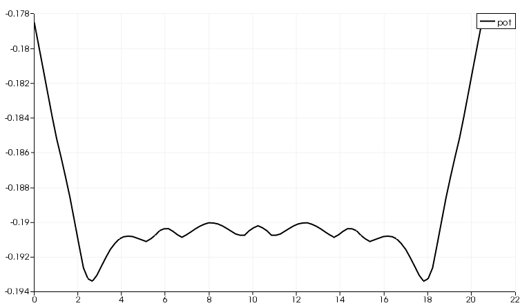
Figure 41 Potential profile along the nanoribbon

As you can notice, there is a discontinuity at the interface. However, it is quite small (~ 12 meV). Defining a ‘perfect’ interface between the bulk semi-infinite contacts and the device region is very difficult, especially in a semiconductor where no free charge can contribute to screen such an interface potential. A smaller tolerance in the self-consistent charge during the contact and the device calculation, a finer calculation of the Fermi level (in metallic systems) and a finer Poisson grid can decrease the discontinuity: you should be able to reach about 1 meV, but it is difficult to go below this value. However, as you can see in the transmission plot, as long as the discontinuity is this small, it hardly affects the transmission.

However, it is important for you to verify that the behaviour at the boundaries is reasonable. Otherwise, the extended region may be too small to allow to the relevant physical quantities (charge, potential) to relax to bulk values. Be aware that numerical errors are unavoidable, therefore it is important to understand their relevance and the impact on the results. In the transmission calculation we do not notice anything different because the energy step is close to the mismatch at the boundaries.

After running the calculation for the pristine system, we will introduce vacancies as we did in the non-SCC calculation. The results should be now directly comparable to the bulk periodic SCC calculation.

SCC armchair nanoribbon with vacancy (A)

[Input: recipes/transport/carbon2d-trans/agr-scc/vacancy1/]

We will now calculate the SCC transmission for the nanoribbon with a vacancy on the sublattice A, using the same input structure set up for the non-SCC calculation. The contacts are identical to the pristine case, therefore in the following we will only modify the extended device calculation.

Transmission and Density of States

As previously done, the transport section must be modified in order to account for the different number of atoms in the extended device region:

Transport {
    Device {
      AtomRange = 1 135
      FirstLayerAtoms =  1 68
    }
    Contact {
      Id = "source"
      AtomRange = 136 271
      FermiLevel [eV] = -4.45
      potential [eV] = 0.0
    }
    Contact {
      Id = "drain"
      AtomRange = 272 407
      FermiLevel [eV] = -4.45
      potential [eV] = 0.0
    }
  Task = UploadContacts {
  }
}

We use the same Fermi level and the files shiftcont_source.dat and shiftcont_drain.dat as in the pristine system calculation, as the contacts are not modified.

The Hamiltonian block is also not modified, except for an additional finite temperature:

Hamiltonian = DFTB {
  ...
  Filling = Fermi {
    Temperature [Kelvin] = 150.0
  }
  ...
}

A finite temperature is used to provide a finite temperature broadening, useful if the vacancy induces partially filled gap states. In general, temperature broadening may improve convergence and dump oscillations in the SCC iterations.

The Analysis block is also similar, we add the DOS calculation to verify if we can identify a vacancy state:

Analysis {
  TunnelingAndDos {
    Verbosity = 101
    EnergyRange [eV] = -6.0  -3.0
    EnergyStep [eV] = 0.025
    Region {
      Atoms = 1:135
    }
  }
}

As usual, you can now create the GS and contacts directories, copy the shiftcont_source.dat and shiftcont_drain.dat in the current directory and run the calculation. The density of states and transmission are shown in Figure Density of states for vacancy (A) and Transmission for vacancy (A).

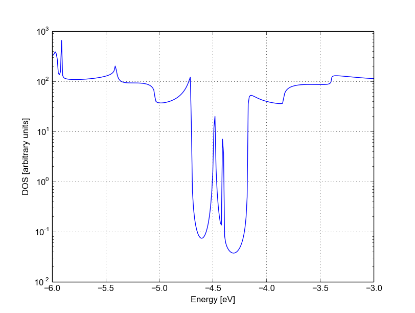
Figure 42 Density of states for vacancy (A)

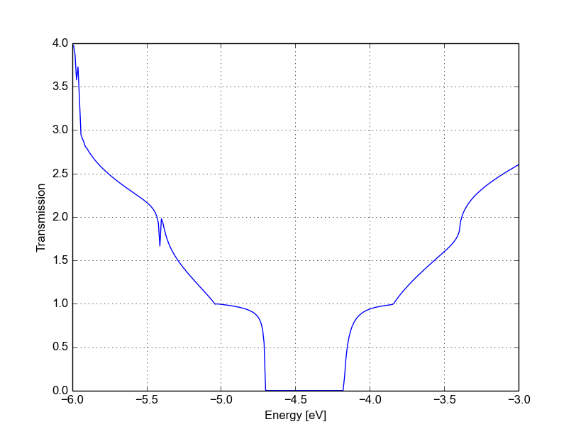
Figure 43 Transmission for vacancy (A)

The vacancy states are located in the energy gap, consistently with the periodic calculation, and that the tunnelling curve is qualitative similar to the non-SCC calculation. The first conduction and valence band are weakly affected by the vacancy which does not act as a strong scatterer. There is no signature of resonances, as the additional levels are located in the gap.

Note also that we previously recommended the use of large extended regions and to verify that the potential and charge density are smooth at interfaces. As you can see in Figure 44, the impurity is very close to the boundaries, resulting to a potential profile which varies significantly close in to the boundary. It is left to the reader to verify that the overall transmission does not change significantly if a longer extended region is considered.

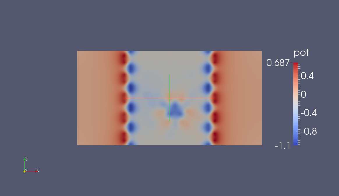
Figure 44 Potential profile for vacancy (A)

SCC armchair nanoribbon with vacancy (B)

[Input: recipes/transport/carbon2d-trans/agr-scc/vacancy2/]

We will now run the same calculation, but with the vacancy on the sublattice B. As in the non-SCC case, the only difference with the previous calculation is the location of the vacancy, therefore the input file is absolutely identical. The contacts are the same, therefore all we have to do is copy the shiftcont_source.dat and shiftcont_drain.dat files into the current directory and run the calculation.

The resulting transmission and density of states are shown in Figures Density of states for vacancy (B) and Transmission for vacancy (B).

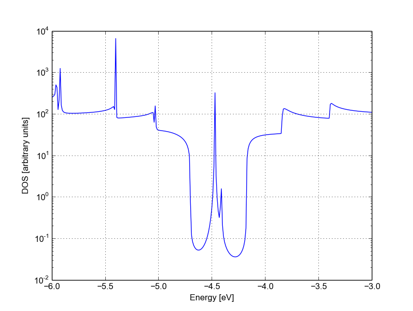
Figure 45 Density of states for vacancy (B)

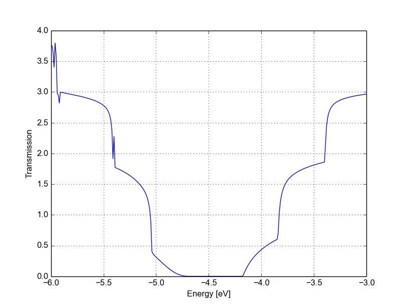
Figure 46 Transmission for vacancy (B)

We immediately notice that the Van Hove singularities are strongly suppressed and that the valence band is substantially suppressed. Consistently with the picture obtained by periodic calculation, a quasi-bounded vacancy level hybridises with the valence band edge causing strong back-scattering. A comparison between all the three cases (see Figure Transmission for pristine system (blue), vacancy (A) (green) and vacancy (B) (red)) shows that the scattering probability is strongly affected by the exact position of the vacancy. This is generally true for other kinds of short range scattering centres in graphene nanoribbons, such as substitutional impurities. We can also notice that in this particular case the non-SCC approximation is qualitatively consistent for two reasons: the vacancy levels are not populated and the charge transfer at the edges is not critical as the edges contribute poorly to the transmission in an armchair ribbon.

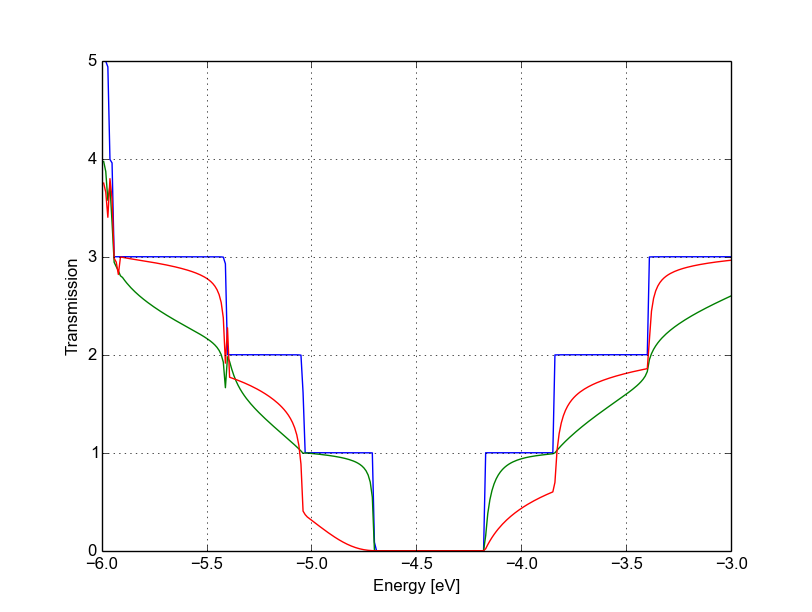
Figure 47 Transmission for pristine system (blue), vacancy (A) (green) and vacancy (B) (red)