Calculation of electronic absorption spectra#
This section discusses the calculation of electronic absorption spectra using the real time propagation of electronic dynamics as implemented in DFTB+.
Unless some good reason exists for not doing so, the electronic spectrum should be calculated at the equilibrium geometry. For this example we will use an optimised chlorophyll a molecule. This example reproduces the results in Oviedo, M. B., Negre, C. F. A., & Sánchez, C. G. (2010). Dynamical simulation of the optical response of photosynthetic pigments. Physical Chemistry Chemical Physics : PCCP, 12(25), 6706–6711.
The input#
[Input: recipes/electronicdynamics/spectrum/]
The following input can be used to calculate the absorption spectrum of chlorophyll a:
Geometry = GenFormat {
  <<< "coords.gen"
}

Hamiltonian = DFTB {
  SCC = Yes
  SCCTolerance = 1.0e-7
  MaxAngularMomentum = {
    Mg = "p"
    C = "p"
    N = "p"
    O = "p"
    H = "s"
  }
  Filling = Fermi {
    Temperature [K] = 300
  }
}

ElectronDynamics = {
   Steps = 20000
   TimeStep [au] = 0.2
   Perturbation = Kick {
     PolarizationDirection = all
   }
   FieldStrength [v/a] = 0.001
}
The optimised geometry is located in the coords.gen file. Note that for this example the long phytol chain present in the natural molecule has been replaced by a terminating hydrogen atom since it does not have a significant influence on the absorption spectrum.
For the calculation of absorption spectra, an initial kick of the system is made using a Dirac delta type perturbation. The input specifies that after the initial perturbation of Kick type, twenty thousand steps of dynamics will be executed using a time step of 0.2 atomic units. The Kick perturbation can be applied in any of the Cartesian directions (x, y or z). The use of all here in the input instructs the code to run three independent dynamic calculations, one with an initial Kick in each Cartesian direction.
After self consistency has been achieved and the ground state density matrix is obtained, the perturbation is applied and then the propagation starts, the output produced is the following:
S inverted
Density kicked along x!
Starting dynamics
Step        0  elapsed loop time:   0.012400  average time per loop   0.012400
Step     2000  elapsed loop time:  19.112000  average time per loop   0.009551
Step     4000  elapsed loop time:  35.407101  average time per loop   0.008850
Step     6000  elapsed loop time:  52.179100  average time per loop   0.008695
Step     8000  elapsed loop time:  68.688004  average time per loop   0.008585
Step    10000  elapsed loop time:  90.615501  average time per loop   0.009061
Step    12000  elapsed loop time: 109.174500  average time per loop   0.009097
Step    14000  elapsed loop time: 127.921097  average time per loop   0.009137
Step    16000  elapsed loop time: 147.406097  average time per loop   0.009212
Step    18000  elapsed loop time: 167.002502  average time per loop   0.009277
Step    20000  elapsed loop time: 185.372406  average time per loop   0.009268
Dynamics finished OK!
S inverted
Density kicked along y!
Starting dynamics
Step        0  elapsed loop time:   0.023700  average time per loop   0.023700
Step     2000  elapsed loop time:  28.003799  average time per loop   0.013995
Step     4000  elapsed loop time:  52.257900  average time per loop   0.013061
Step     6000  elapsed loop time:  74.137497  average time per loop   0.012354
Step     8000  elapsed loop time:  93.527603  average time per loop   0.011689
Step    10000  elapsed loop time: 115.045998  average time per loop   0.011503
Step    12000  elapsed loop time: 134.955200  average time per loop   0.011245
Step    14000  elapsed loop time: 155.862000  average time per loop   0.011132
Step    16000  elapsed loop time: 176.434799  average time per loop   0.011026
Step    18000  elapsed loop time: 197.430695  average time per loop   0.010968
Step    20000  elapsed loop time: 217.860703  average time per loop   0.010892
Dynamics finished OK!
S inverted
Density kicked along z!
Starting dynamics
Step        0  elapsed loop time:   0.012100  average time per loop   0.012100
Step     2000  elapsed loop time:  27.119101  average time per loop   0.013553
Step     4000  elapsed loop time:  48.640301  average time per loop   0.012157
Step     6000  elapsed loop time:  67.843803  average time per loop   0.011305
Step     8000  elapsed loop time:  87.514702  average time per loop   0.010938
Step    10000  elapsed loop time: 111.822601  average time per loop   0.011181
Step    12000  elapsed loop time: 133.397202  average time per loop   0.011116
Step    14000  elapsed loop time: 153.044098  average time per loop   0.010931
Step    16000  elapsed loop time: 176.008301  average time per loop   0.011000
Step    18000  elapsed loop time: 195.700104  average time per loop   0.010872
Step    20000  elapsed loop time: 216.208694  average time per loop   0.010810
Dynamics finished OK!
The resulting time dependent dipole moment along each Cartesian direction produced the kicks are stored in the mu*.dat output files.
The calculation of the spectrum makes use of the fact that the Fourier transform of induced dipole moment of the molecule in the presence of an external time dependent field (within the linear response range) is related to the Fourier transform of said field in the following manner:
\(\mathbf{mu}(\omega)=\overset\leftrightarrow{\alpha}(\omega)\mathbf{E}(\omega)\)
since the Fourier transform of a Dirac delta is a constant at all frequencies, the polarizability tensor \(\overset\leftrightarrow{\alpha}(\omega)\) can be obtained from the time dependent response. The absorption is proportional to the imaginary part of the trace of the polarizability tensor.
The calculation of the absorption spectrum is carried out using the script
calc_timeprop_spectrum either available after make install of DFTB+, or
located in the tools/misc directory under the dftbplus source tree. The
invocation of the script is as follows:
calc_timeprop_spectrum -d 20.0 -f 0.001
The exciting field strength is specified with the -f flag, the -d flag specifies a damping constant used to exponentially damp the dipole signal to zero within the simulation time. This damping time is expressed in femtoseconds. The effect of damping the dipole moment is to add a uniform width to every spectral line and is necessary to smooth out any ringing in the spectrum peaks after the transform. In essence this damping procedure is equivalent to using a windowing function.
The spectrum is located in the output files spec-ev and spec-nm. In this case the spectrum looks as follows:
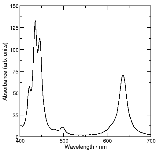
The band between 400 and 500 nm is called the Soret band and the one between 600 and 700 nm is the Q band. This band is the band that provides is responsible for the photo-biologic activity of chlorophylls as antennae capable of capturing solar energy in the primary process of photosynthesis.