In the simplest case, transport calculations can be performed on an atomistic
structure comprising of two semi-infinite contacts. These contacts are usually
one-dimensional periodic systems (wire-like) and connect to a device region.
In order to carry out a transport calculation with DFTB+, the geometry of the
system must be carefully partitioned by the user and the structure must
contain:
The extended molecule (the central region),
Two Principal Layers (see below) for the first contact,
Two Principal Layers of the second contact.
(additional contacts can also be included, but we will first start with the most
common situation of a 2 contact geometry).
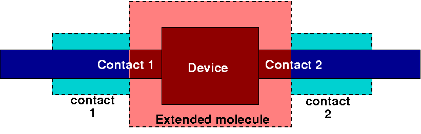
Figure 25 Partitioning of a simple system into an extended molecule and perfect
contacts.#
The extended molecule contains the atomistic device itself plus those parts of
the attached contacts, which are directly influenced by the presence of the
device (we can call them surfaces). Each contact, on the other hand, contains
those parts of the actual contacts, which are far enough from the device not to
be affected by it (the examples below will better clarify this point).
The most important concept to bear in mind is that of principal layers (PLs).
These are defined as contiguous groups of atoms that have interaction only with
atoms of the immediately adjacent PLs. In practice these layers must contain a
sufficient number of atoms in order to ensure that the hamiltonian and overlap
interactions vanish before reaching the second nearest neighbour PLs (or can be
considered negligible). The subdivision of the system into PLs is essential for
the definition of the two contacts and becomes useful in the computation of all
Green’s functions that exploit a recursive algorithm (See [PPD2008]).
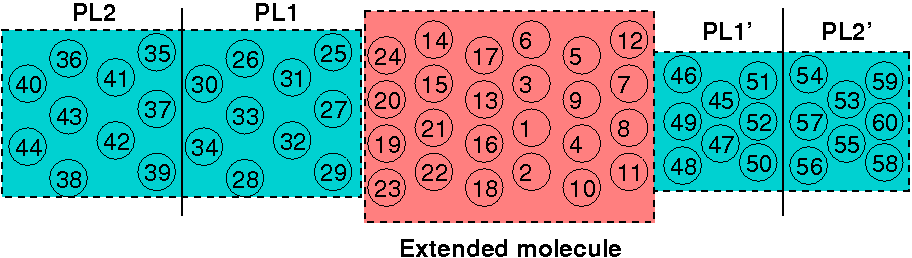
Figure 26 Subdivision of a general structure into principal layers (PL), two for each
contact and an arbitrary number within the extended molecule region.#
As shown in Figure 26, the extended
device molecule can contain an arbitrary number of PLs (>=1), but the layers
themselves must follow a sequential ordering. The ordering of the PLs follow
directly from the spatial ordering of the atoms in the DFTB+ structure.
Typically it is convenient to create the structure and then sort the atom along
the transport direction before then partitioning up the system. In other cases,
for example when nanowires are constructed, it is more convenient to repeat a PL
unit for the desired length of the extended molecule.
The (perfect) contacts are defined by two principal layers. Unlike the layers of
the extended molecule region, the PLs defining the contacts must follow
additional rules:
The two principal layers of a given contact must be identical.
They must be rigidly shifted images of each other.
The first PL must be the closest to the device region.
In order to ensure that the above prescriptions are met the numbering of the
atoms must follow a precise ordering.
The atoms of the central region must be specified first in the structure,
i.e. before the atoms of the contacts (see Partitioning the system and contacts for
details). The atoms of each of the contacts then follow those of the central
region in turn. The atoms of each contact must be grouped together sequentially
(You specify either all atoms of the left contact first, and then those of the
right one, or vice versa). The numbering field for the atoms in the gen format
input is ignored (see Geometry for details), it is the order of the
atoms in the structure that matters. We often find it useful for readability to
number atoms in the device (or its principal layers) sequentially, then restart
the count for each contact.
The numbering of the atoms within the first principal layer of a contact is
arbitrary, but the same ordering of atoms must be applied to the second PL of
that contact. Thus, the order that the atoms are listed in each of the two
contact PLs must be the same and their location in the list must differ by the
same amount for all atoms in the two PLS. The coordinates of the equivalent
atoms in the two layers must also differ by the same vector (the contact
vector) which translates all atoms of the first PL onto their equivalents in
the second PL. These prescriptions are checked by DFTB+ and an error message is
issued if the two PLs do not conform to these requirements. It is important to
remember to number the atoms of the first PL to be the layer closer to the
device, i.e. they must contain the atoms with the lowest indices in the contact.
Figure 27 Example for numbering of the atoms. Those in the device have the lowest
indices, followed by the atoms of each contact, respectively. The two
principal layers making up each contacts are shifted copies of each other
(both in space and order of numbering).#
DFTB+ can compute transport for structures that have periodicity in one or both
directions that are transverse with respect to the transport direction. In this
case the structure must be defined as a supercell and the rules listed above
apply to the resulting cell. The real-space Poisson solver of DFTB+ limits the
supercell lattices to being of orthorombic type (orthogonal vectors parallel to
the cartesian axes, i.e. all angles between supercell vectors must be 90
degrees). In fact the supercell is always defined as being 3-dimensional, and
the user should ensure that the dummy lattice vector along the transport
direction is long enough to avoid superpositions between atoms in images along
that direction.
The current version of DFTB+ only supports one supercell definition for the
entire system, including central region and contacts. It may be redundant to
observe that in this case the two contacts must be of the same periodicity in
the directions transverse to the transport direction.
The geometry must be defined in the transport block, as specified in the
following example:
Transport{Device{# Device is the 1st to 24th atom in the geometry listAtomRange=124}Contact{Id="source"# This contact starts at atom 25AtomRange=2544}Contact{Id="drain"# This contact starts at atom 45AtomRange=4558}}