Calculations using range-separated TD-DFTB#
In DFT there are a variety of exchange-correlation functionals, for example the local density approximation (LDA) or various gradient corrected functionals (GGA). Functionals that mix pure DFT and HF, so-called hybrid functionals are widely used in chemistry and physics. A new member of the club are the range-separated (or long-range corrected) functionals that combine pure DFT for short electron-electron distance with HF at longer distance. Conventional DFTB is based on the GGA, while ground and excited state calculations for range-separated functionals are now also available in DFTB+. The corresponding method is named LC-DFTB.
You will need a recent version of DFTB+ (>= 21) to perform the calculations in this section.
Benzene-Tetracyanoethylene dimer (TD-DFTB)#
[Input: recipes/linresp/range-separated/td-dftb]
Let us first do a conventional TD-DFTB calculation for the dimer of tetracyanoethylene (TCNE) and a benzene molecule to show the difference between both approaches. Here is the relevant part of the input:
Hamiltonian = DFTB {
    SCC = Yes
    SCCTolerance = 1.0E-10
    MaxAngularMomentum = {
       N = "p"
       C = "p"
       H = "s"
    }
    SlaterKosterFiles = Type2FileNames {
        Prefix = "../../../slakos/download/mio/mio-1-1/"
        Separator = "-"
        Suffix = ".skf"
    }
}

ExcitedState {
    Casida {
        NrOfExcitations = 10
        Symmetry = Singlet
        Diagonaliser = Stratmann {SubSpaceFactor = 30}
    }
}
We are loading here the mio Slater-Koster files, which have been
generated using the GGA functional PBE. Note the new entry
Diagonalizer in the Casida block. Besides the default Arpack
diagonalizer also the Stratmann algorithm may be used for the
diagonalization of the response matrix. For small systems like the
present one, the Stratmann option is very often faster.
The output in EXC.DAT looks like follows:
    w [eV]       Osc.Str.         Transition         Weight      KS [eV]    Sym.

================================================================================

   2.033        0.00000000        37   ->    38        1.000       2.033      S
   2.035        0.00000031        36   ->    38        1.000       2.035      S
   3.162        0.00000000        35   ->    38        1.000       3.162      S
   3.164        0.00000000        34   ->    38        1.000       3.164      S
   4.346        0.00000054        32   ->    38        1.000       4.346      S
   4.524        0.39252514        33   ->    38        1.000       3.442      S
   4.570        0.00000000        31   ->    38        1.000       4.570      S
   4.573        0.00000000        30   ->    38        1.000       4.573      S
   4.881        0.00000000        29   ->    38        1.000       4.881      S
   4.897        0.00000000        28   ->    38        1.000       4.897      S
The lowest excited state at 2.033 eV corresponds to the HOMO->LUMO transition. We can visualize these orbitals using waveplot (see First steps with Waveplot) to obtain more information on the nature of this state (Figure 21 and Figure 22).
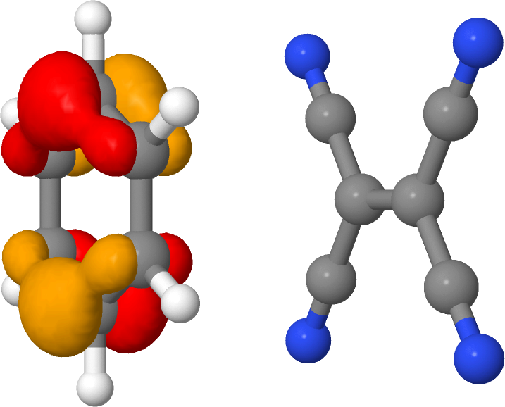
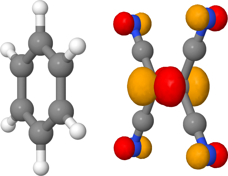
We see that the lowest excited state is of charge transfer type, in which an electron is excited from the donor (benzene) to the acceptor (TCNE). TD-DFT using GGA functionals typically strongly underestimates such states, and this is also the case for TD-DFTB.
Benzene-Tetracyanoethylene dimer (TD-LC-DFTB)#
[Input: recipes/linresp/range-separated/td-lc-dftb]
We now repeat the calculation using the TD-LC-DFTB method. The input looks like this:
Geometry = GenFormat {
    <<< "in.gen"
}

Driver = {}

Hamiltonian = DFTB {

    SCC = Yes
    SCCTolerance = 1.0E-10
    MaxAngularMomentum = {
        N = "p"
        C = "p"
        H = "s"
    }
    SlaterKosterFiles = Type2FileNames {
        Prefix = "../../../slakos/download/ob2/ob2-1-1/shift/"
        Separator = "-"
        Suffix = ".skf"
    }
    RangeSeparated = LC {
        Screening = MatrixBased {}
    }
}

ExcitedState {
    Casida {
        NrOfExcitations = 10
        Symmetry = Singlet
        Diagonaliser = Stratmann {SubSpaceFactor = 30}
    }
}
TD-LC-DFTB requires special Slater-Koster files that have been
generated for range-separated functionals. We are loading the ob2
set here. The block RangeSeparated invokes the LC-DFTB method for
the ground state. Several algorithms to speed up the calculation are
available (see manual), we are choosing the MatrixBased algorithm
here which involves no approximations. The ExcitedState section
requires no changes, although the Stratmann diagonalizer is
mandatory for TD-LC-DFTB. As you will recognize, the calculation is
slower than the previous TD-DFTB job. You can play with the parameter
SubSpaceFactor (c.f. manual) to see the influence on the execution
time.
Let us now investigate the output (EXC.DAT) of the job:
  w [eV]       Osc.Str.         Transition         Weight      KS [eV]    Sym.

================================================================================

  4.287        0.00000000        37   ->    38        1.000       6.748      S
  4.290        0.00000013        36   ->    38        1.000       6.751      S
  4.930        0.51883432        33   ->    38        1.000       7.719      S
  4.962        0.00000101        35   ->    38        1.000       7.389      S
  4.963        0.00000002        34   ->    38        1.000       7.391      S
  5.257        0.00000000        32   ->    38        1.000       9.063      S
  5.263        0.00000000        29   ->    38        1.000       9.117      S
  5.595        0.00000000        28   ->    38        1.000       9.377      S
  5.860        0.00000000        27   ->    38        1.000       9.646      S
  6.018        0.00000000        24   ->    38        0.999       9.790      S
The lowest excited state is shifted from 2.033 eV (TD-DFTB) to 4.287 eV (TD-LC-DFTB). If you visualize the relevant molecular orbitals with waveplot, you can verify that the nature of the state is indeed unchanged, but the severe underestimation is corrected!