Solvation effects#
Chemistry mainly happens in the condensed phase in solvation. To model this environment effect we can employ an implicit solvation model.
Partition coefficients#
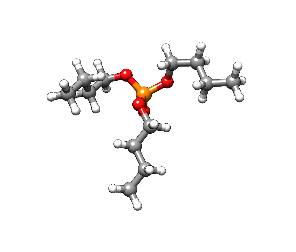
We will again use the tributyl phosphate system for this chapter starting from the lowest conformer computed at DFT level of theory.SGS+22
44

P            0.04979860695690        0.44711451464043       -1.00582935088785
O           -1.01828570201577        1.61992081924505       -1.08204989992478
O            1.44541819964837        1.20259350968357       -0.93004646393268
O           -0.23116449461962       -0.19092086100911        0.43348057584036
O            0.04989811059549       -0.52939857862507       -2.13193727489898
C           -3.22595849860852        0.57569749292020       -0.63048371070980
C            3.17125059294208        2.26919500606264        0.37793012664706
C           -0.49671006005934       -2.62276723852782        0.51752296451488
C           -2.37291235771157        1.37377084394425       -1.59520657808180
C            1.69082363056085        2.25168490238616        0.06491515604763
C            0.42423494323872       -1.45148539577987        0.79538479831033
C           -3.40028045343485        1.23959706437998        0.73452517731784
C            3.66251230954912        1.00475672173489        1.08259311966198
C            0.14365149763826       -3.95555023713892        0.91118196598503
C           -4.25721021459863        0.39844726585583        1.67794675785264
C            5.14863386178168        1.07197599507234        1.42894858037114
C           -0.77275034832669       -5.13994447582840        0.60668692357785
H           -4.20593926439767        0.44583117295978       -1.11148258102692
H           -2.80524727780564       -0.43169945847273       -0.50895563008287
H            3.73396375795546        2.42972141752258       -0.55124157858279
H            3.35560124098091        3.14584756668454        1.01426453778633
H           -1.43320670149735       -2.47989437852294        1.07245708104755
H           -0.74649279399252       -2.63205125963662       -0.55075018369840
H           -2.28435686339904        0.87349896173282       -2.56570622164894
H           -2.77764831943878        2.37852774636938       -1.74559624331743
H            1.10045874685666        2.04089452960540        0.96551158716685
H            1.35623984857714        3.19828298483888       -0.37219697034341
H            0.64786384718387       -1.35765077566991        1.86259993322524
H            1.37041338393201       -1.54864147188351        0.24797788513280
H           -3.85688415770214        2.22927316800735        0.59672718397360
H           -2.41375306800835        1.40599090456599        1.18221915186467
H            3.47264091184327        0.13643034401191        0.44003684602247
H            3.07393423247992        0.85408789825825        1.99820770460226
H            0.39073192854148       -3.94380191866237        1.98125890567555
H            1.09263532764405       -4.07715111779153        0.37207018493030
H           -3.79637849612223       -0.58020445552568        1.85370039309811
H           -4.38030266458304        0.88988483294634        2.64812230808074
H           -5.25489295914165        0.22661390262107        1.25834559004993
H            5.47806835596330        0.16138801918681        1.93896808119261
H            5.75695498422814        1.18910728560937        0.52530220715744
H            5.36133224641826        1.92201274229434        2.08696405672930
H           -1.00459785333360       -5.18748938484018       -0.46299441722211
H           -0.30604962300523       -6.08751382128645        0.89294337567665
H           -1.71987305808669       -5.05272568826932        1.15031517963084
For a partition coefficient we need to evaluate the solvation free energy for the two phases, we will evaluate the environmental relevant octanol-water partition coefficient (logKow). The formula for the partition coefficients can needs the free energies for the molecule in water and octanol
Tip
The value \(\log e / (k_B T)\) at 298 K is 460.200 Eh–1.
We will setup a calculation using the ALPB solvation model,ESSG21 using the GFN2-xTB and DFTB3-D4 using the inputs below for water.
Geometry = xyzFormat {
<<< "struc.xyz"
}

Hamiltonian = xTB {
  Method = "GFN2-xTB"
  Solvation = GeneralizedBorn { ParamFile = solvation/gfn2-1-0/param_alpb_water.txt }
}

Options = { WriteDetailedOut = No }
Analysis { CalculateForces = Yes }
ParserOptions = { ParserVersion = 10 }
Parallel = { UseOmpThreads = Yes }

Driver = GeometryOptimization {}
Geometry = xyzFormat {
<<< "struc.xyz"
}

Hamiltonian = DFTB {
  SCC = Yes
  MaxAngularMomentum {
    H = "s"
    C = "p"
    O = "p"
    P = "d"
  }
  HubbardDerivs {
    H = -0.1857
    C = -0.1492
    O = -0.1575
    P = -0.1400
  }
  ThirdOrderFull = Yes
  HCorrection = Damping { Exponent = 4.0 }
  SlaterKosterFiles = Type2FileNames {
    Prefix = "slakos/3ob-3-1/"
    Separator = "-"
    Suffix = ".skf"
  }
  Dispersion = DFTD4 {
    s6 = 1.0
    s9 = 0.0
    s8 = 0.4727337
    a1 = 0.5467502
    a2 = 4.4955068
  }
  Solvation = GeneralizedBorn { ParamFile = solvation/3ob-1-0/param_alpb_h2o.txt }
}

Options = { WriteDetailedOut = No }
Analysis { CalculateForces = Yes }
ParserOptions = { ParserVersion = 10 }
Parallel = { UseOmpThreads = Yes }

Driver = GeometryOptimization {}
Exercise
Perform the calculation for the free energy of water and octanol. You might need to adjust the parameter file name for the octanol solvent parameters.
How well does the calculated partition coefficient compare to the experimental value of 4.0? Is the value well reproduced, which effects are not accounted for?
Summary#
You learned…
to setup an implicit solvation model with DFTB and xTB
perform an optimization accounting for solvation effects
calculate a partition coefficient from free energies