Waveplot is a tool for generating grid-based volumetric data for charge
distributions or wave-functions in your system. By visualising those
distributions with appropriate graphical tools you can obtain a deeper
understanding of the physics and chemistry of your quantum mechanical system.
In order to plot the charge distribution or the orbitals in a certain system,
you have to execute a DFTB+ calculation for this system first. The calculation
must be executed as usual, you just have to make sure, that the options
WriteDetailedXML and WriteEigenvectors are turned on.
Below you see the input for the H2O molecule, where the geometry is
optimised by DFTB+:
Running DFTB+ for this input, you should obtain the usual results, and
additionaly the files detailed.xml and eigenvec.bin. Former contains
some information about the calculated system, latter contains the obtained
eigenvectors in binary format. Both files are needed by waveplot.
Now, you have to decide, what kind of charge distributions, wavefunctions etc.
to plot. In the current example, we will plot the total charge distribution of
the water molecule, the charge distribution (wavefunction squared) for the
highest occupied molecular orbital (HOMO), the wave function for the HOMO, and
the total charge difference, which tells us, how the chemical bonding between
the atoms modified the total charge distribution compared to the superpositions
of neutral atomic densities.
The appropriate waveplot input (waveplot_in.hsd) could look like the
following:
# General options

Options {
  TotalChargeDensity = Yes           # Total density be plotted?
  TotalChargeDifference = Yes        # Total density difference plotted?
  ChargeDensity = Yes                # Charge density for each state?
  RealComponent = Yes                # Plot real component of the wavefunction
  PlottedSpins = 1 -1
  PlottedLevels = 4                  # Levels to plot
  PlottedRegion =  OptimalCuboid {}  # Region to plot

  NrOfPoints = 50 50 50              # Number of grid points in each direction
  NrOfCachedGrids = -1               # Nr of cached grids (speeds up things)
  Verbose = Yes                      # Wanna see a lot of messages?
}

DetailedXml = "detailed.xml"         # File containing the detailed xml output
                                     # of DFTB+
EigenvecBin = "eigenvec.bin"         # File cointaining the binary eigenvecs


# Definition of the basis
Basis {
  Resolution = 0.01
  # Including mio-1-1.hsd. (If you use a set, which depends on other sets,
  # the wfc.*.hsd files for each required set must be included in a similar
  # way.)
  <<+ "../../slakos/wfc/wfc.mio-1-1.hsd"
}
Some notes to the input:
Option TotalChargeDensity controls the plotting of the total charge
density. If turned on, the file wp-abs2.cube is created.
Option TotalChargeDifference instructs Waveplot to plot the difference
between the actual total charge density and the density you would obtain by
summing up the densities of the neutral atoms.
Option ChargeDensity tells the code, that the charge distribution for some
orbitals (specified later) should be plotted. Similarly, RealComponent
instructs Waveplot to create cube files for the real part of the one-electron
wavefunctions for the specified orbitals. (For non-periodic systems the
wavefunctions are real.)
Options PlottedSpins, PlottedLevels (for periodic systems also
PlottedKPoints) controls the levels (orbitals) to plot. In the current
example we are plotting level 4 (is the HOMO of the water molecule) for all
available spins. Since the DFTB+ calculation was spin unpolarised, we obtain
only one plot for the HOMO in file wp-1-1-4-abs2.cube (1-1-4 in the file
name indicates first K-point, first spin, 4th level).
The region to plot is selected with the option PlottedRegion. Instead of
specifying the box origin and box dimensions by hand, Waveplot can be
instructed by using the OptimalCuboid method to take the smallest cuboid,
which contains all the atoms and enough space around them, so that the
wavefunctions are not leaking out of it. (For details and other options for
PlottedRegion please consult the manual.) The selected region in the
example is sampled by a mesh of 50 by 50 by
50. (NrOfPoints)
The basis defintion (Basis) is made by including the file containing the
appropriate wave function coefficient definitions. You must make sure that
you use the file for the same set, which you used during your DFTB+
calculation. Here, the mio-1-1 set was used for calculating the H2O
molecule, and therefore the file wfc.mio-1-1.hsd is included.
The wavefuntion coefficients can be usually downloaded from the same place as
the Slater-Koster files.
================================================================================
     WAVEPLOT  0.2
================================================================================

Interpreting input file 'waveplot_in.hsd'
--------------------------------------------------------------------------------
WARNING!
-> The following 3 node(s) had been ignored by the parser:
(1)
Path: waveplot/Basis/C
Line: 1-33 (File: wfc.mio-0-1.hsd)
(2)
Path: waveplot/Basis/N
Line: 52-84 (File: wfc.mio-0-1.hsd)
(3)
Path: waveplot/Basis/S
Line: 120-170 (File: wfc.mio-0-1.hsd)

Processed input written as HSD to 'waveplot_pin.hsd'
Processed input written as XML to 'waveplot_pin.xml'
--------------------------------------------------------------------------------

Doing initialisation

Starting main program

Origin
  -5.00000 -6.35306 -6.47114
Box
  10.00000 0.00000 0.00000
  0.00000 11.08472 0.00000
  0.00000 0.00000 12.94228
Spatial resolution [1/Bohr]:
  5.00000 4.51071 3.86331

Total charge of atomic densities:    7.981973


 Spin KPoint  State  Action        Norm   W. Occup.
    1      1      1    read
    1      1      2    read
    1      1      3    read
    1      1      4    read

Calculating grid

    1      1      1    calc    0.996855    2.000000
    1      1      2    calc    1.003895    2.000000
    1      1      3    calc    0.998346    2.000000
    1      1      4    calc    1.000053    2.000000
File 'wp-1-1-4-abs2.cube' written
File 'wp-1-1-4-real.cube' written
File 'wp-abs2.cube' written

Total charge:    7.998297

File 'wp-abs2diff.cube' written

================================================================================
Some notes on the output:
The warnings about unprocessed nodes appears, because the included file
wfc.mio-0-1.hsd also contained wave function coefficients for elements (C,
N, S), which are not present in the calculated system. Hence these extra
definitions in the file were ignored.
The Totalchargeofatomicdensities tells you the amount of charge found
in the selected region, if atomic densities are superposed. This number should
be approximately equal to the number of electrons in your system (here 8).
There could be two reasons for a substantial deviation. Either the grid is not
dense enough (option NrOfPoints) or the box for the plotted region is too
small or misplaced (PlottedRegion).
The output files for the individual levels (charge density, real part,
imaginary part) follow the naming convention wp-KPOINT-SPIN-LEVEL-TYPE.cube.
The total charge and the total charge difference are stored in the files
wp-abs2.cube and wp-abs2diff.cube, respectively.
The volumetric data generated by Waveplot is in the Gaussian cube format and can
be visualized with several graphical tools (VMD, JMol, ParaView, …). Below we
show the necessary steps to visualize it using VMD. (It refers to VMD version
1.8.6 and may differ in newer versions.)
The cube file containing the total charge distribution wp-abs2.cube can be
read by using the File|NewMolecule menu. VMD should automatically
recognise, that the file has the Gaussian cube format. After successful loading,
the VMD screen shows the skeleton of the molecule.
In order to visualise the charge distribution, the graphical representation of
the molecule has to be changed. This can be achieved by using the
Graphics|Representations... submenu. The skeleton representation can be
turned to a CPK represenation (using balls and sticks) by selecting CPK for the
Drawingmethod in the GraphicalRepresentations dialog box. Then you
should create an additional representation (CreateRep) and change the
drawing method for it to be Isosurface. The type of isosurface (Draw)
should be changed from Points to SolidSurface and instead of
Box+Isosurface only Isosurface should be selected. Then, by tuning the
Isovalue one can select the isosurface to be plotted.
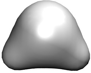
Figure 1 was created using 0.100. (Display background
color had been set to white using the Graphics|Colors menu.)
Figure 1 Total charge density for the H2O molecule, created by Waveplot, visualised
by VMD.#
The charge distribution difference can be plotted in a similar way as the total
charge. One has to load the file wp-abs2diff.cube. One should then, however,
make not one, but two additional graphical representations of the type
Isosurface. One of them should have positive isovalue, the other one a
negative one. The different isosurfaces can be colored in a different way by
using ColorID as coloring method and choosing different color values for the
different representations.
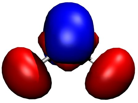
Figure 2 demonstrates this for the water
molecule. Negative net populations were colored red, positive net populations
blue. One can clearly see, that there is a significant electron transfer from
the hydrogens to the oxygen (lone pair on the oxygen).
Figure 2 Charge density difference (total density minus sum of atomic densities) for
the H2O molecule, as created by Waveplot and visualised by VMD.#
The plotting of molecular orbitals can be, depending which property is plotted,
done in the same way as the total charge distribution or the total charge
difference. If the charge density (probability distribution) of an orbital is
plotted, the data contains only positive values, therefore only one isosurface
representation is necessary (like for the charge distribution). If the real (or
for periodic systems also the imaginary) part of the wavefunction is to be
plotted, two isosurface representations are needed, one for the positive and one
for the negative values (like for the charge difference).
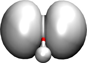
Figure 3 shows the distribution of the electron
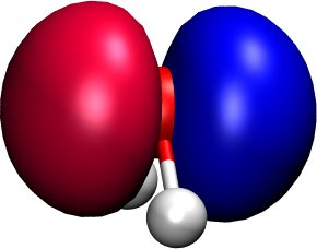
(wavefunction squared) for the HOMO, while Figure 4
shows the HOMO wavefunction itself (blue - positive, red - negative). You can
easily recognise the p-type of the HOMO, positive on one side, negative on the
other side, a node plane in the middle.
Figure 3 Highest occupied molecular orbital of a water molecule (wavefunction
square)#
Figure 4 Highest occupied molecular orbital of a water molecule (real part of the
wavefunction).#