Geometry relaxation in the excited state#
So far we have only looked at excited state calculations at fixed geometry. DFTB+ supports also geometry relaxations or even MD simulations in a given excited state. In this example we are going to study the absorption and fluorescence energies of the simple molecule thioformaldehyde (\({SCH}_2\)).
Thioformaldehyde absorption#
[Input: recipes/linresp/range-separated/relax/abs]
We are starting with a geometry that has already been relaxed in the ground state. Performing a TD-DFTB calculation at this geometry yields the following spectrum (EXC.DAT):
w [eV]       Osc.Str.         Transition         Weight      KS [eV]    Sym.

================================================================================

    1.848        0.00000000         6   ->     7        1.000       1.848      S
    4.770        0.10134777         5   ->     7        0.999       3.837      S
    5.077        0.00000000         4   ->     7        1.000       5.077      S
    5.467        0.00126721         6   ->     8        1.000       5.457      S
    6.000        0.00000000         3   ->     7        1.000       6.000      S
    7.128        0.00006156         6   ->     9        1.000       7.128      S
    7.138        0.00000000         6   ->    10        1.000       7.138      S
    7.327        0.02861414         6   ->    11        1.000       7.224      S
    7.446        0.00000000         5   ->     8        1.000       7.446      S
    8.964        0.08762770         4   ->     8        1.000       8.685      S
Note that we are only interested in singlet states here, since absorption to triplet states is spin forbidden. We will focus on the first excited state (\({S}_1\)).
Thioformaldehyde absorption#
[Input: recipes/linresp/range-separated/relax/abs]
We are starting with a geometry that has already been relaxed in the ground state. Performing a TD-DFTB calculation at this geometry yields the following spectrum (EXC.DAT):
w [eV]       Osc.Str.         Transition         Weight      KS [eV]    Sym.

================================================================================

    1.848        0.00000000         6   ->     7        1.000       1.848      S
    4.770        0.10134777         5   ->     7        0.999       3.837      S
    5.077        0.00000000         4   ->     7        1.000       5.077      S
    5.467        0.00126721         6   ->     8        1.000       5.457      S
    6.000        0.00000000         3   ->     7        1.000       6.000      S
    7.128        0.00006156         6   ->     9        1.000       7.128      S
    7.138        0.00000000         6   ->    10        1.000       7.138      S
    7.327        0.02861414         6   ->    11        1.000       7.224      S
    7.446        0.00000000         5   ->     8        1.000       7.446      S
    8.964        0.08762770         4   ->     8        1.000       8.685      S
Note that we are only interested in singlet states here, since absorption to triplet states is spin forbidden. We will focus on the first excited state (\(S_1\)) at 1.848 eV, which has symmetry \(A_2\). This symmetry can be inferred by inspection of the molecular orbitals involved in the transition, but we will not do so in this recipe. The state at 4.77 eV has much larger oscillator strength, but in real life also the \(S_1\) state will be very weakly absorbing due to electron-phonon coupling. This is however not taken into account at the present level of theory. Due to symmetry, the oscillator strength is exactly zero in our example.
Adiabatic excitation energies#
[Input: recipes/linresp/range-separated/relax/emi]
We now relax the structure in the first excited state. The input (dftb_inp.hsd) for this task looks like this:
Geometry = GenFormat {
    <<< "in.gen"
}

Driver = LBFGS {}

Hamiltonian = DFTB {

    SCC = Yes
    SCCTolerance = 1.0E-10
    MaxAngularMomentum = {
        S = "d"
        C = "p"
        H = "s"
    }
    SlaterKosterFiles = Type2FileNames {
        Prefix = "../../../slakos/download/mio/mio-1-1/"
        Separator = "-"
        Suffix = ".skf"
    }
}

ExcitedState {
    Casida {
        NrOfExcitations = 10
        StateOfInterest = 1
        Symmetry = Singlet
        Diagonaliser = Stratmann {SubSpaceFactor = 30}
    }
}

ParserOptions = {
    ParserVersion = 10
}
In contrast to the earlier examples in this recipe, we now set a
Driver. We choose LBFGS optimization, but one could also take any
other optimizer available in DFTB+. You may also set convergence
criteria for the forces like detailed in the recipe
Basic usage. Important is the new entry in the Casida block
StateOfInterest. It tells the code to optimize on the \(S_1\)
potential energy surface. It is recommended to choose
NrOfExcitations always somewhat larger (i.e., +5) as
StateOfInterest, since iterative eigensolvers might not converge to
the exact solution for boundary eigenvalues. Note also that during a
relexation the order of the excited states might change. This is a
frequent cause of error in these kind of simulations.
You should see that the geometry optimization finishes in a few steps. Visualizing the relaxed structure shows that the S-C bond length increased by 0.5 Angstroem. The experimental value for the bond length in the \(S_1\) is 1.68 Angstroem. What do you get?
During the optimization, the file EXC.DAT is constantly updated. Let us have a look at the final result:
   w [eV]       Osc.Str.         Transition         Weight      KS [eV]    Sym.

================================================================================

   1.738        0.00000000         6   ->     7        1.000       1.738      S
   4.512        0.10509561         5   ->     7        0.999       3.516      S
   4.846        0.00000000         4   ->     7        1.000       4.846      S
   5.386        0.00097579         6   ->     8        1.000       5.379      S
   5.915        0.00000000         3   ->     7        1.000       5.915      S
   7.157        0.00000000         5   ->     8        1.000       7.157      S
   7.204        0.00005764         6   ->     9        1.000       7.204      S
   7.215        0.00000000         6   ->    10        1.000       7.215      S
   7.445        0.01593134         6   ->    11        1.000       7.384      S
   8.818        0.10121357         4   ->     8        1.000       8.487      S
We see that the excitation energy of the \(S_1\) decreased by 0.11 eV. This value corresponds to the so-called Stokes shift, which measures the difference between absorption and fluorescence energies. In the present example, absorption and radiative de-excitation from the \(S_1\) (i.e., fluorescence) should be very difficult to detect, as already mentioned above. The following diagram illustrates the energetic landscape:
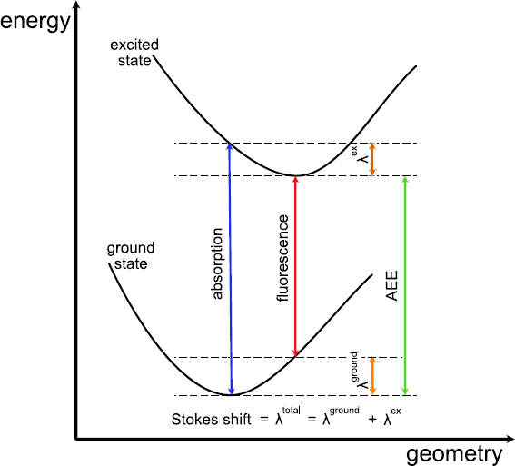
Figure 23 Sketch of the adiabatic excitation energy (AEE), reorganization energies \(\lambda\) in the ground and excited states, and Stokes shift [Taken from Sokolov et al., JCTC 17, 2266 (2021)]#
We will now compute the adiabatic excitation energy. As the diagram Figure 23 shows, this requires the ground state energies of the starting structure and the relaxed structure. We can get these from the respective detailed.out files. The experimental value is 2.03 eV, what do you get?