Example: Molecular Junction#
[Input: recipes/transport/molecular-junction/]
This example guides in the definition of a contact/molecule/contact geometry for transport calculations.
Tasks 0: Preparing the structure#
Before starting any calculation it is necessary to define the structure following the rules given in the section, Specifying the geometry. Here we give some tips in order to speed up the process. The following procedure is valid for systems with 2 contacts placed along the same transport direction.:
It is convenient to initially define a structure without paying attention to its atom ordering. The system should be complete, with each contact comprising two PLs.
Once the structure has been prepared, convert it to a simple xyz format file
Reorder the atoms according to the coordinates along the transport direction. In Linux this can be achieved using sort, e.g.,
$ sort -n -k
2 input.xyz > output.xyz
This will sort according to ‘column #2’, corresponding to the ‘x’ coordinates. Even better, the following command line will skip the first two lines$ (head -2 input.xyz && tail -n +3 input.xyz | sort -nk 2) > output.xyzCheck that, after sorting, the contacts comprise of 2 PLs with exactly the same atomic ordering (see Setup Geometry utility if you only have 1 PL).
Open the sorted xyz structure with a text editor and move the first contact to the end of the list of atoms. After this place the atoms of the second PL, the first PL must be closer to the device region.
Reconvert back to gen format (xyz2gen) and add the supercell information, if present.
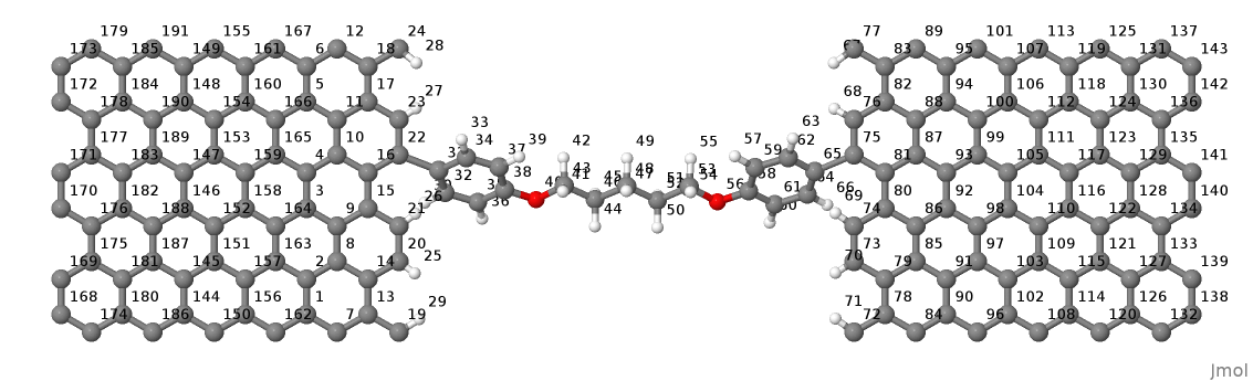
Figure 62 System with atoms sorted along the x-direction.#
Now the system is ready for transport calculations. It is possible to define PLs
also in the molecular (device) region, which can be quite useful for speeding up
calculations. The size of these PLs depends on the largest cutoff in the
tight-binding interactions. Figure _fig_transport_junction-sort-col shows
an example of PLs highlighted in different colours.
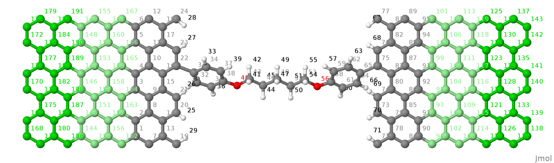
Figure 63 System showing the different PLs highlighted with colours.#
Relaxation of the structure#
Only the molecular atoms were allowed to move, namely the first 95 atoms in the list. The contact regions must be kept fixed. The definition of the two PLs, as rigid shifted copies of each other, will otherwise be lost. It is a good idea to build the contact PLs from previously relaxed bulk structures.
In setting up the example structure, we found it a bit difficult to relax at first since the SCC-loop did not converge. In such cases it is better to proceed in a sequence of different relaxation steps.:
Initially the structure was optimised with a non-SCC calculation and just Gamma point sampling.
More k-points where added in the direction y, parallel to transport (for this geometry the structure periodically repeats along this direction, but not along z due to the large vacuum gap for this supercell). Then re-relaxed.
SCC was finally switched on and the structure re-relaxed from the final non-SCC geometry.
In order to help SCC convergence and avoid electrostatic artefacts, the dangling bonds at both contact ends have been saturated with hydrogen atoms. In other cases, if the system allows, it is possible to initially optimise a periodic supercell which repeats along the transport direction (but where any contact atoms are kept fixed). It is then possible to relax under open boundary conditions, but this can be left as a final refinement step.
Task 1: Calculation of the contacts#
In the input file you need to specify the Geometry and Transport blocks for the contact calculations tasks:
Geometry = GenFormat {
<<< str.gen'
}
Transport {
  Device {
    AtomRange = 1 95
  }
  Contact {
    Id = "Source"
    AtomRange = 96 143
    PLShiftTolerance = 0.01
  }
  Contact {
    Id = "Drain"
    AtomRange = 144 191
    PLShiftTolerance = 0.01
  }
  Task = ContactHamiltonian{
     ContactId = "Source"
  }
}
Notice the tag PLShiftTolerance added here, since in this case the 2 contact
PLs are not perfect rigid copies of each other. It is possible to comment
out this tag and see the error message from DFTB+.
With task ContactHamiltonian DFTB+ performs a contact calculation. The code
extracts, from the complete device geometry, the contact defined with Id =
"Source" and constructs appropriate supercell vectors from the coordinates
given in the two PLs. The rest of the input file refers to a standard DFTB+
calculation of a supercell system, for which an appropriate k-point sampling
must be specified:
Hamiltonian = DFTB {
SCC = Yes
MaxAngularMomentum {
C = "p"
O = "p"
H = "s"
}
SlaterKosterFiles = Type2FileNames{
Prefix = "./mio-1-1/"
Separator = "-"
Suffix = ".skf"
}
Filling = Fermi{
Temperature [Kelvin] = 0.0
}
# Appropriate for transport along x, periodic along y and a vacuum gap on z:
KpointsAndWeights = SupercellFolding {
16 0 0
0 4 0
0 0 1
0.5 0.5 0.5
}
}
Contact supercell#
Since in this example the input geometry is defined as a supercell, DFTB+
preserves the meaningful supercell vectors. In this case the transport direction
is along x and the relevant periodicity is along the lateral direction, y.
The supplied supercell vector along x is dummy as the structure is open in
that direction, whereas the periodicity along z defines the graphene-graphene
separation. This z value does matter in the definition of the Poisson Box
(see below) so cannot be made arbitrarily large. The DFTB+ code internally
builds a supercell vector for the contact along the x-direction, taken from
the geometry definition of the two PLs. Hence, the contact computation is
performed for the two PLs of the contact and results are saved in
shiftcont_source.dat for later use. For this reason it is recommended to
set appropriate values for the k-point sampling in all directions. In this
particular case we can set 1 k-point along z, since this is a dummy
periodicity, but both x and y should be convergently sampled (note that in
this example the contact region the cell is shorter along x than y so will
probably require more k-points).
An appropriate k-sampling is important in order to converge the Fermi energy and
contact shift calculations. It is possible to experiment by changing the number
of k-points and check the convergence of the SCC-charges and Fermi energy in
detailed.out.
After the “Source” contact has been computed, you must change the input file and carry out a similar computation for the “Drain” contact.
Task 2: SCC Calculation of the device in equilibrium#
The SCC calculation of transport usually starts with an equilibrium calculation of the system with open-boundary conditions.
The Transport section must be modified:
Transport {
Device {
AtomRange = 1 95
FirstLayerAtoms = 1, 21, 43, 54
}
Contact {
Id =
"Source"
AtomRange = 96 143
PLShiftTolerance = 0.01
FermiLevel [eV] = -4.665975
Potential [eV] = 0.0
}
Contact {
Id = "Drain"
AtomRange = 144 191
PLShiftTolerance = 0.01
FermiLevel [eV] = -4.665975
Potential [eV] = 0.0
}
}
Here it is important to note the value of FermiLevel which is taken from the
contact calculations as reported in the files shiftcont_source/drain.dat.
In case of identical contacts the Fermi levels will both be exactly the
same. In this case the two contacts are sightly different resulting in a tiny
difference of Fermi levels. Given the very small difference and in order to
avoid complications that will be discussed in another tutorial, we have forced
both Fermi levels to an averaged value.
The contact potentials are set to 0.0 in order to start from an equilibrium calculation.
The keyword FirstLayerAtoms is used for the definition of the principal
layers in the extended molecule of the device region. As the name of the keyword
suggests, the principal layers are defined by specifying the first atom of each
layer as described above (Task 0).
Poisson solver options#
For the transport calculation the default GammaFunctional solver is
substituted with the Poisson solver:
Electrostatics = Poisson {
  MinimalGrid [Angstrom] = 0.4 0.4 0.4
  AtomDensityTolerance = 1e-5
  CutoffCheck = Yes
  BuildBulkPotential = No
  SavePotential = Yes
  PoissonAccuracy = 1e-5
}
The tag Poisson is used to define the size of the Poisson box domain. The
Poisson equation is solved via a real-space multigrid solver that employs
finite-differences for discretisation on a finite box with a regular grid
(structured mesh). The charge density on the right-hand-side is constructed
exactly as in standard gamma-functional of DFTB, namely expanding the charge
density into spherical s-like atomic densities weighted by atomic Mulliken
charges.
The real-space box size is obtained in this example from the supercell definition. The box length along the transport direction is constrained by the position of the contacts and is internally adjusted.
The Poisson equation is solved with the following boundary conditions (BC):
Dirichelet or mixed BC on the faces containing contacts.
Neumann BC on the remaining faces.
The meaning of the additional options for the Poisson tag are the following:
MinimalGrid = 0.4 0.4 0.4is used to specify that the grid must be spaced at less than 0.4 Ang. in all dimensions. The actual grid is adjusted internally since the number of grid points in every direction must be a power of 2 (exactly \(N = 2^n + 1\)).
AtomDensityTolerance = 1e-5is used to specify, where the exponential decaying spherical s-like atomic charge densities should be cut off. Specifying a certain value here makes sure that all atoms contributing a density higher than the given value are considered when calculating the amount of charge at a certain point (default: 1e-5). The appropriate cutoff radius for that tolerance is calculated automatically by the code (and reported in the output). It is determined by finding the cutoff distance for each atom (\(\alpha\)), where the s-like charge density
\[n_\alpha(r) = \frac{\tau_{\alpha}^3}{8 \pi} e^{-\tau_{\alpha}r}\]becomes smaller than the given tolerance. Then the maximal cutoff found for all atom types in the system is used. The quantity \(\tau_{\alpha}= \frac{16}{5} U_{\alpha}\) is the relationship between the extinction coefficient and the Hubbard parameter in atomic units (see [EPJE1998]).
In order to have a consistent calculation, the determined cutoff length must be smaller than the width of the principal layers when doing a calculation with contacts. The program will check for this criterion and stop if it is not fulfilled. In this example we set it exactly to the default value, only for clarification purposes.
CutoffCheckif set to
No, the code omits the check at to whether the cutoff for the atomic densities (either determined byAtomDensityToleranceor directly set byAtomDensityCutoff) is larger than the widths of the principal layers in the contacts. Please note that a cutoff bigger than the width of any contact PL results in inconsistent calculation, so turning this check off is highly discouraged, unless you exactly know what you are doing. (for experts only)BuildBulkPotential = Nois used to specify that at the device/contact interfaces the bulk potential must be imposed as BCs. The bulk potential is computed for an ideal contact (infinite wire, sheet or surface). Here we should remind you that a key assumption in transport calculations is that the contacts are in equilibrium and that the device/contact interfaces are sufficiently far from the device with enough extended molecule contact-like material such that bulk conditions are recovered. This means that the charge density and potential at this interface should smoothly join with the bulk values. Setting this flag to Yes is important whenever there is a charge redistribution within the contact atoms that has an effect on the bulk potential, like in structures of heteronuclear species (e.g. SiC, GaAs, ZnO, etc.). In the case of graphene there is no charge redistribution between atoms hence the contact potential is 0, so its calculation is not necessary.
Green’s function options#
Here we discuss the most important parameters to be set in the calculation of the system Green’s functions:
Solver = GreensFunction {
  Delta [eV] = 1e-4
  ContourPoints = 30 40
  RealAxisStep [eV] = 0.025
  EnclosedPoles = 0
}
The Green’s function approach is used to compute the density matrix directly for the system and as such it does not solve the eigenproblem (no eigenvectors are computed, hence no band structure is available).
ContourPointsis used to specify the number of quadrature points in the contour integration (see also DFTB+ manual for a description of the complex contour). The default 20 20 has been increased here in order to improve convergence.
Deltadefines a small imaginary number used in the computation of the Green’s function. The default is usually fine.
EnclosedPolesis set to 0 when the temperature is low (T=0). For T>0 few poles (usually 3) needs to be included within the contour.
Task 3: Bias calculations#
Contact potentials can be set in order to put the system under bias. In this example we have performed 3 calculations by setting different contact potentials, hence total biases of 0.0, 0.5 V and 1.0 V:
# A bias of 0.5 V between contacts
Contact {
  Id = "Source"
  Potential [eV] = -0.250
}
Contact {
  Id = "Drain"
  Potential [eV] = 0.250
}
Notice that we set a symmetric bias on the junction, but this is not necessary.
Also notice that in order to set a potential in volts it is necessary to specify
energy units of eV.
When the system is biased, the Green’s function calculation also requires points along the energy axis on the bias window.
RealAxisStepIs used to specify the point sampling along the real axis. The value was set in order to have 20 points for the bias of 0.5 V and 40 points at 1.0 V. The default step is 1500 points/Hartree, corresponding to about 0.018 eV.
RealAxisPointsAlternatively, it is possible to set directly the number of points using this tag.
Notice that at finite temperatures the real axis integration extends by a
certain multiple of kT beyond the bias window. This is essentially due to
the tail of the Fermi function. It is instead possible to set the cutoff
directly in units of kT, using the keyword FermiCutoff.
Critical values and convergence issues#
Open BC calculations are not at all trivial. Convergence can be slow and is usually slower than supercell or cluster calculations. This happens because charge fluctuations within the central region (remember this calculation is in the Grand Canonical Ensemble) makes convergence of the SCC loop harder. Whenever convergence issues are encountered the user should consider trying the following points
Increase the number of ContourPoints, especially the second number.
Decrease the Poisson MinimalGrid: values between 0.2 and 0.4 are usually fine.
Decrease the BroydenMix parameter (MixingParameter = 0.05 or 0.02 can help).
Compute with the Temperature > 0.
Finite temperature calculations can be quite useful when there are partially
filled states, since these tend to oscillate wildly around the Fermi energy
preventing convergence. The temperature can be progressively decreased by
restarting calculations and reading previously computed charges
(ReadInitialCharges=Yes).
Results: Analysis block#
The output of the calculation is reported in the file detailed.out. The file
contains the same information of traditional DFTB+ calculations. However, since
the Green’s functions solver does not find eigenvalues and eigenvectors, some
values are not shown.
In order to calculate the transmission probability between contacts or the
density of states the Analysis block must be specified:
Analysis{
  TunnelingAndDos{
    verbosity = 0
    EnergyRange [eV] = -9.0 -2.0
    EnergyStep [eV] = 0.02
    Delta [eV] = 1e-4
  }
}
As a post SCC calculation, the transmission across the device is computed. This
is accomplished by defining the TunnelingAndDos block. EnergyRange
Defines the energy range for the transmission plot EnergyStep Defines the
interval sampling step.
The code will output files like transmission.dat which contain the
transmission as a two column dataset, this can then can be plotted for example
with xmgrace.
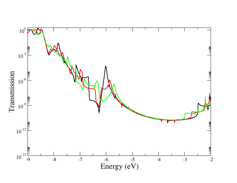
Figure 64 Transmission function for the graphene/molecule/graphene system.#