Benchmarking and scalability#
If you want results more rapidly, it is important to work out approximately how many compute processors to use to calculate your problem (particularly if there is a per-processor cost for using that resource). Just using the maxium available number of cores may be inefficient, so benchmarking a “typical” example of your calculation can help to get results faster and avoid wasting resources.
Your test examples should be large enough to require more than a trivial amount of computer time to be run due to inaccuracies in timing short calculations:
* Random variations in processor/network load can produce noise in
  the times

* You might want to run your tests several times on the same
  platform and average the timings
If your aim is to run large problems, you can use tests on small “toy” versions and estimate resource requirement for the big cases to be feasibly simulated.
Timers#
DFTB+ has an internal timer for various significant parts of its calculations. This can be enabled by adding the following option to the input:
Options {
  TimingVerbosity = 2
}
This will activate the timers for the most significant stages of a calculation. Higher values increase the verbosity of timing, while a value of -1 activates all available timers.
The typical output of running the code with timers enabled for a serial calculation will end with lines that look something like
--------------------------------------------------------------------------------
DFTB+ running times                          cpu [s]             wall clock [s]
--------------------------------------------------------------------------------
Pre-SCC initialisation                 +     3.46  (  5.8%)      3.45  (  5.8%)
SCC                                    +    47.34  ( 79.6%)     47.34  ( 79.6%)
  Diagonalisation                           44.79  ( 75.3%)     44.79  ( 75.3%)
  Density matrix creation                    2.21  (  3.7%)      2.21  (  3.7%)
Post-SCC processing                    +     8.68  ( 14.6%)      8.68  ( 14.6%)
  Energy-density matrix creation             0.55  (  0.9%)      0.55  (  0.9%)
  Force calculation                          7.74  ( 13.0%)      7.74  ( 13.0%)
  Stress calculation                         0.94  (  1.6%)      0.94  (  1.6%)
--------------------------------------------------------------------------------
Missing                                +     0.00  (  0.0%)      0.00  (  0.0%)
Total                                  =    59.48  (100.0%)     59.47  (100.0%)
--------------------------------------------------------------------------------
This shows the computing time (cpu) and real time (wall clock) times of major parts of the calculation.
An alternative method to obtain total times is by using the built-in shell command time when running the DFTB+ binary
time dftb+ > output
In the above example, at the termination of the code timings will be printed:
real    0m59.518s
user    0m59.430s
sys     0m0.092s
More advanced timing is possible by using profiling tools such as gprof.
Examples#
Shared memory parallelism#
The strong scaling for the OpenMP parallel code for some example inputs is shown here
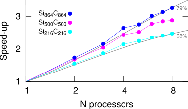
These results were calculated on an old Xeon workstation (E5607 @ 2.27GHz) and are a self-consistent calculation of forces for different sized SiC supercells with 1 k-point and s and p shells of orbitals on the atoms. Timings and speed-ups come from data produced from the code’s reported total wall clock time.
There are several points to note
The parallel scalability improves for the larger problems, going from ~68% to ~79% on moving from 512 atoms to 1728. This is a common feature, that larger problems give sufficient material for parallelism to work better.
The gain in throughput for these particular problems is around a factor of 2 when using 4 processors, and raises to around 3 on 8 processors for the largest problem.
From Amdhal’s law we can estimate the saturating speed-up limits for large numbers of processors as ~3.1 and ~4.8 for the smallest and largest problems respectively. This implies that there is not much value in using more than ~4 processors for the smallest calculation, since this has already gained around 2/3 of its theoretical maximum speed up on 4 processors. Adding a 5th or 6th processor will only improve performance by ~5% each, so is probably a waste of resources. Similarly for the largest calculation in this example, 6 processors gives around a factor of 3 speed up compared to serial operation, but adding 7th processors will only speed the calculation up by a further ~6%.
The experimental data does not align exactly with the Amdahl curves, this could be due to competing processes taking resources (this is a shared memory machine with other jobs running) or the problem may run anomalously well for a particular number of processes. In this example 4 processors consistently ran slightly better, perhaps due to the cache sizes on this machine allowing the problem to be stored higher in the memory hierarchy for 4 processors compared to 3 (thus saving some page fetching).
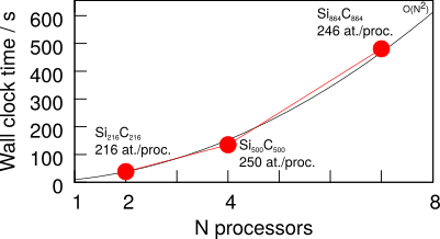
The weak scaling (increasing the number of processors proportional to the number of atoms) shows an approximately \(O(N^2)\) growth in time. A serial solution of these problems would increase as \(O(N^3)\) in the number of atoms.
These timings are for this specific hardware and these particular problems, so you should test the case you are interested in before deciding on a suitable choice of parallel resources.
Weak scaling from the same data set is shown here
Spin locks#
[Input: recipes/parallel/spinlock/]
The idealised performance of Amdahl’s law assumes that the parallel parts of the calculation can be spread over arbitrarily large numbers of computing units without any contention between them.
In reality, finite problems can only be meaningfully broken down to some lower limit of sub-problem size. Similarly, operations that require different processes to cooperate can find them waiting for each other to complete (an example of spinlock/contention behaviour), then release the resulting data with the latency of moving it around between different levels of the memory hierarchy.
This leads in practice to the performance of a calculation actually degrading if too many processors are requested. This will depend on the particular hardware and libraries being used.
Below are examples for an excited state calculation of a C60 molecule using OpenMP parallelism. See the Linear response excitations section for details about this type of calculation.
In this example, being too greedy in requesting processes leads to worse parallelism (or even a slower calculation):
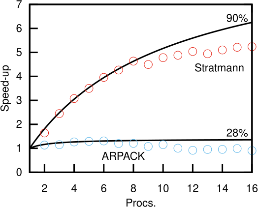
As you can see, the ARPACK solver is not a very parallel calculation (28%). There is some marginal improvement in throughput up to ~4 processes. But, beyond this point it rapidly becomes not just inefficient, but counter-productive to add more processors to try and get your results faster. The Stratmann solver is better (90% parallel in this case), but even there, above ~8 processors, the parallelism degrades.
Of course, this doesn’t actually tell you which solver is faster to get the answer to the problem, only how they scale. To find this out requires comparing the actual wall-clock times:
Procs |
ARPACK |
Stratmann |
1 |
38.31s |
106.96s |
6 |
29.32s |
27.03s |
8 |
31.76s |
23.07s |
As you can see, on one processor the ARPACK solver is actually faster (the Stratmann solver is currently optimized for finding only a few excited states, and this example calculates 100). By 6 processors (the last point ARPACK shows any speed-up for this example), this speed advantage is lost while Stratmann continues getting faster (being ~1.7x faster to get the solution than serial ARPACK when using 8 processors,).
The above data was generated from the Post-SCC processing wall clock time printed by DFTB+, which is dominated by the excited state calculation in this case. The number of Open MP threads is varied with the relevant shell variable:
export OMP_NUM_THREADS=1
dftb+
export OMP_NUM_THREADS=4
dftb+
You can also use the system timer time dftb+, but the internal timers produce a more finegrained output of timings
DFTB+ running times                          cpu [s]             wall clock [s]
--------------------------------------------------------------------------------
Global initialisation                  +       0.00 (  0.0%)       0.01 (  0.0%)
SCC                                    +       0.15 (  0.4%)       0.19 (  0.5%)
  Diagonalisation                              0.13 (  0.3%)       0.18 (  0.5%)
Post-SCC processing                    +      38.23 ( 99.6%)      38.31 ( 99.5%)
--------------------------------------------------------------------------------
Missing                                +       0.00 (  0.0%)       0.00 (  0.0%)
Total                                  =      38.38 (100.0%)      38.52 (100.0%)
--------------------------------------------------------------------------------
Distributed memory parallelism#
This section coming soon!
Topics to be discussed:
Parallel scaling of simple examples.
Parallel efficiency.
Use of the Groups keyword in DFTB+ to improve scaling and efficiency for calculations with spin polarisation and/or k-points.
Effects of latency on code performance.
GPU computing#
Description coming soon!