NEB via File-IO

[Input: recipes/interfaces/ase/neb/fileio/]

In order for ASE to find the DFTB+ executable and Slater-Koster files, environment variables must be set. Assuming the use of the BASH shell, this is done as follows (in general an adaptation to your specific computing environment will be necessary):

$ DFTB_PREFIX=~/slakos/mio-0-1/
$ DFTB_COMMAND=~/dftbplus/bin/dftb+

Geometry

To calculate the energy barrier of the umbrella inversion process, it is necessary to provide geometries for the initial and final state.

A possible choice for the .gen files defining the initial and final state of the calculation could be the following:

initial state:

  4  C
N  H
  1 1    0.3282523436E+00   -0.6075947736E+00    0.1062852063E+00
  2 2    0.1193013364E+01   -0.3265926020E+00    0.5715962197E+00
  3 2    0.2770647466E+00   -0.1801902091E+00   -0.8199941035E+00
  4 2   -0.4767004541E+00   -0.3215324152E+00    0.6662026774E+00

final state:

  4  C
N  H
  1 1    0.3206429517E+00   -0.6319775238E+00    0.1527307910E+00
  2 2    0.1179077740E+01   -0.1010702015E+01    0.5563961495E+00
  3 2    0.2628891413E+00   -0.8794981362E+00   -0.8365549890E+00
  4 2   -0.4905898328E+00   -0.1001302325E+01    0.6515180485E+00

Figure 62 visualizes the defined geometries. The NH₃ molecule passes through a planar transition state, thus inverting the pyramidal shape:

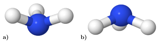
Figure 62 Initial a) and final b) state of the NH₃ (ammonia) umbrella inversion.

Main script

The Python script shown below is a suitable and simple implementation to run a calculation with NIMAGES as the number of intermediate images (in this case set to 13).

The main method then first reads in the geometry and immediately writes it out for the reasons mentioned in Socket-Comm.: Geometry Optimization by ASE. The trajectories (obtained from previous calculations) of the initial and final state are read in and a list with the individual images is created, whereby the first and last image is determined by the states that have just been read in. True, independent copies of the first image are created for the 13 intermediate images. A NEB object is instantiated and a linear interpolation of the path from the intial and final state is calculated.

Subsequently, the ASE driver BFGS() for geometry optimization is specified and where to write the resulting trajectory (i2f.traj). A list of instantiated DFTB calculators is created and its elements attached to the single intermediate images. Finally the calculation is started by calling the run command, while passing the maximum force component fmax (mind the ASE Units!):

from ase.io import read, write
from ase.neb import NEB
from ase.optimize import BFGS
from ase.calculators.dftb import Dftb

NIMAGES = 13

def main():
    '''Main driver routine.'''

    initial = read('NH3_initial.traj')
    final = read('NH3_final.traj')

    images = [initial]
    images += [initial.copy() for ii in range(NIMAGES)]
    images += [final]

    neb = NEB(images)
    neb.interpolate()

    opt = BFGS(neb, trajectory='i2f.traj')

    calcs = [Dftb(label='NH3_inversion',
                  Hamiltonian_SCC='Yes',
                  Hamiltonian_SCCTolerance='1.00E-06',
                  Hamiltonian_MaxAngularMomentum_N='"p"',
                  Hamiltonian_MaxAngularMomentum_H='"s"')
             for ii in range(NIMAGES)]

    for ii, calc in enumerate(calcs):
        images[ii + 1].set_calculator(calc)

    opt.run(fmax=1.00E-02)


if __name__ == "__main__":
    main()

Analysis

The results of the NEB calculation can be extracted out of the trajectory file i2f.traj using corresponding ASE tools. If only the last 15 images (intermediate images plus initial and final state) are of interest, a construction like the following one would be suitable:

ase gui i2f.traj@-15:

Since ASE is capable of quickly visualizing the reaction path via the Tools ‣ NEB tab, you should obtain something similar to Figure 63:

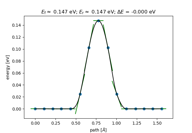
Figure 63 Energy barrier of the umbrella inversion of a single NH₃ (ammonia) molecule.

Since the initial and final state are identical after a suitable unitary transformation, the energetic difference \(\Delta E\) between the states obviously vanishes.