Band structure, DOS and PDOS#
This chapter demonstrates, using the example of anatase (TiO2), how the band structure, density of states (DOS) and the partial density of states (PDOS) of a periodic system (such as wires, surfaces or solids) can be obtained using DFTB+.
The conversion scripts used here are part of the dptools package, which is distributed with DFTB+. In order to perform the calculations in this chapter, you will need the Slater-Koster sets mio and tiorg. The sample input files assume that the necessary Slater-Koster files have been copied into a subdirectory mio-ext.
Introduction#
The calculation of the band structure for a periodic system consists of two steps.
First for self-consistent (SCC) calculations, the charges in the system must be calculated using a converged k-point sampling.
Then, keeping the obtained self-consistent charges fixed, the one-electron levels must be calculated for k-points chosen along the specific lines in k-space of the chosen band structure. These are usually between high symmetry points in the Brillouin zone of that unit cell.
Creating the proper input charges#
[Input: recipes/basics/bandstruct/1_density/]
In order to calculate a band structure in Density Functional Theory (DFT), at first the ground-state density for the given system must be obtained. In the DFTB picture, this corresponds to obtaining the self-consistent charges of the atoms. These charges must be convergent with respect to two quantities in order to give correct results:
Tolerance of the SCC cycle and
quality of the k-point sampling grid.
In the current tutorial, the SCC tolerance is set to be 1e-5. For the
k-point sampling, the \(8 \times 8 \times 8\) Monkhorst-Pack set will be
used. Both quantities ensure good convergence in the charges for anatase, but
may not be suitable for other applications.
We will also use the results of the converged calculation to obtain information about the density of states (DOS) and the partial density of states (PDOS) of anatase. This information only makes sense when extracted from a system with a good k-point sampling. A sample dftb_in.hsd input looks like:
Geometry = GenFormat {
    6  F
 Ti  O
    1 1    0.4393045491E-02   -0.4394122690E-02   -0.4185505032E-06
    2 1   -0.2456050838E+00   -0.7543932244E+00    0.5000007729E+00
    3 2    0.1997217007E+00    0.2106836749E+00   -0.1813953963E-02
    4 2   -0.4625010039E+00    0.4843137675E-01    0.4981557672E+00
    5 2   -0.2106822274E+00   -0.1997223911E+00    0.1816384188E-02
    6 2   -0.4843281768E-01   -0.5374990457E+00    0.5018414482E+00
    0.0000000000E+00    0.0000000000E+00    0.0000000000E+00
   -0.1903471721E+01    0.1903471721E+01    0.4864738245E+01
    0.1903471721E+01   -0.1903471721E+01    0.4864738245E+01
    0.1903471721E+01    0.1903471721E+01   -0.4864738245E+01
}

Hamiltonian = DFTB {
  Scc = Yes
  SccTolerance = 1e-5
  SlaterKosterFiles = Type2FileNames {
    Prefix = "../../../slakos/mio-ext/"
    Separator = "-"
    Suffix = ".skf"
  }
  MaxAngularMomentum {
    Ti = "d"
    O  = "p"
  }
  KPointsAndWeights = SupercellFolding {
    4 0 0
    0 4 0
    0 0 4
    0.5 0.5 0.5
  }
}

Analysis {
  ProjectStates {
    Region {
      Atoms = Ti
      ShellResolved = Yes
      Label = "dos_ti"
    }
    Region {
      Atoms = O
      ShellResolved = Yes
      Label = "dos_o"
     }
  }
}

ParserOptions {
  ParserVersion = 12
}
In the input above, the coordinates have been specified in relative (fractional)
coordinates, which express the positions of the atoms as a linear combination of
the lattice vectors. This is indicated by using the letter F in the first
line of the geometry specification:
Geometry = GenFormat {
    6  F
 :
The k-points are generated automatically using the SupercellFolding
method, which enables among others the generation of Monkhorst-Pack schemes. In
the current example, a k-point set equivalent to the Monkhorst-Pack scheme
\(4 \times 4 \times 4\) has been chosen (For details how to specify the
coefficients and the shift vectors, please consult the manual).:
KPointsAndWeights = SupercellFolding {
  4 0 0
  0 4 0
  0 0 4
  0.5 0.5 0.5
}
You can check, by generating denser k-point sets, that the current choice gives an accuracy in the range of 1e-3 eV for the total energy. Also, by specifying a smaller SCC tolerance than the chosen one (1e-5) you can check that converging the charges more precisely does not significantly decrease the total energy. We note in passing that these settings provide well converged results for the total energy in the current example, but in principal may not provide converged values for other properties. One should, in principal, test the convergence of any evaluated properties with respect to the calculation parameters.
We will plot the DOS of this system by using the output in the file
band.out. In order to also obtain a PDOS as well, the appropriate atoms (on to
which the electronic states should be projected) are also specified. The
resulting data will then be stored in separate files. In practice, this is done
in the Analysis block using the ProjectStates options. In our example:
Analysis {
  ProjectStates {
    Region {
      Atoms = Ti
      ShellResolved = Yes
      Label = "dos_ti"
    }
    Region {
      Atoms = O
      ShellResolved = Yes
      Label = "dos_o"
     }
  }
}
we decide to get the PDOS for the Ti and the O atoms separately. Each Region
block specifies the atoms (either selected by species, atomic ranges, or as a
combination of both), for which PDOS should be created. Additionally, you can
select, whether you would like to see each atomic shell of the atoms in a region
(s, p, d, etc.) separately or together for that region. With the Label tag
you can specify the prefix for the data files created. Using the settings above,
we will obtain 5 files: dos_ti.1.dat, dos_ti.2.dat, dos_ti.3.dat,
dos_o.1.dat and dos_o.2.dat. The first three contain the PDOS for the s, p,
and d shells of Ti, while the last two files provide the oxygen s and p shells.
Plotting the density of states#
You can use the dp_dos program from the dptools package to take the eigenlevels stored in band.out, apply a gaussian smearing to them, and to store the result in a format, which can be easily plotted by any 2D visualization tool. You have to issue:
dp_dos band.out dos_total.dat
This would create a file dos_total.dat in NXY format, with the energies as X-values and the calculated DOS values as Y-values. You can tune the output by setting different options for dp_dos. Invoke it with the help option:
dp_dos -h
shows detailed information about possible options. The results can be visualised with xmgrace, for example, with the commands:
xmgrace -nxy dos_total.dat
and by zooming into the region around the Fermi-level (showing the valence band edge and the conduction band edge), you should obtain a picture like this:
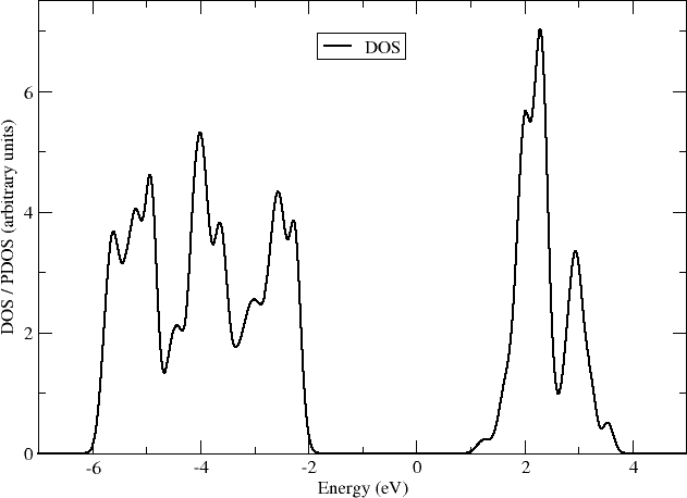
In order to investigate the nature of the states forming the valence and conduction band edges, we will then plot the contribution of the individual atomic shells to the band edges. For that, we have to convert the PDOS-files into NXY files. In the case of dos_ti.1.dat you would execute:
dp_dos -w dos_ti.1.out dos_ti.s.dat
and similarly for the other PDOS files. It is important that you specify the
weighting option -w for the PDOS files, as otherwise the total DOS (instead
of the appropriate PDOS) will be created in each case. By visualizing the
obtained data files together with the total DOS, you should obtain a picture
like:
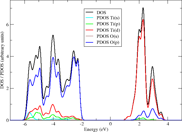
Here you can see that the valence band edge of anatase is entirely composed of the oxygen p-orbitals, while the conduction band edge is made of the d-orbitals of titanium.
Calculating the band structure#
[Input: recipes/basics/bandstruct/2_bands/]
Once well converged charges for a system have been obtained, the band structure can then be calculated at any chosen k-point. In our case, we will choose the points lying along a line which goes through the high symmetry points, Z-Gamma-X-P, of the anatase Brillouin zone. In order to do that, the input has to be changed slightly:
# ...

Hamiltonian = DFTB {
  Scc = Yes
  ReadInitialCharges = Yes
  MaxSCCIterations = 1

  # ...

  KPointsAndWeights = Klines {
    1   0.5   0.5  -0.5    # Z
   20   0.0   0.0   0.0    # G
   45   0.0   0.0   0.5    # X
   10   0.25  0.25  0.25   # P
  }
}

# ...
Note: only the relevant parts of the input are shown, here. See the Introduction section on how to obtain the archive with the full input.
The input is (must be) almost the same as in the previous case, with only a few adaptions:
As we want to use the charges, as obtained in the previous well converged calculation, you have to copy the charges.bin file from the previous calculation into the directory of the current calculation. At the same time, you must instruct the code to read those charges, by setting:
ReadInitialCharges = Yes
Since we want to use the well converged charges to obtain the band structures and do not want to change them during the calculation, the maximal number of SCC cycles should be set to 1:
MaxSCCIterations = 1
Finally, the k-points should be adapted according to the lines in the Brillouin-zone, along which you wish to obtain the band structure. You can achieve that by using the Klines directive:
KPointsAndWeights = Klines {
  1   0.5   0.5  -0.5    # Z
 20   0.0   0.0   0.0    # G
 45   0.0   0.0   0.5    # X
 10   0.25  0.25  0.25   # P
}
Every line of this block specifies a line segment. The first column gives the number of k-points along the line segment between (but excluding) the end of the previous line segment and the k-point which is specified as the next three columns (which is the end point of the current line segment). The specified number of k-points are evenly distributed along the line segment, with the last k-point coincident with the end point of the segment. The coordinates of the k-points are fractional coordinates (given in the coordinate system of the reciprocal lattice vectors of the periodic structures).
The starting point of the first line segment is by default the Gamma point, but you can override this behaviour by setting a first line segment with one point only, as demonstrated above for the Z-point.
Running DFTB+ with the input above, the eigenlevel spectrum is calculated at the required k-points. The results are written to the file band.out. You can use the script dp_bands from the dptools package to convert this file into XNY format. By issuing:
dp_bands band.out band
you would then obtain a file band_tot.dat containing the band structures. After plotting it, you should see something like:
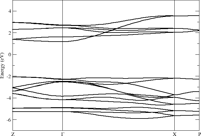
Note, DFTB+ enumerates the k-points along the lines you specified starting at one. The vertical bars corresponding to the special points \(Z\), \(\Gamma\), \(X\) and \(P\) must be therefore inserted on positions 1, 21, 66, 76.