The DFTB+ distribution includes a tool to help prepare structures for transport
calculations in accordance with the requirements described in
Specifying the geometry. Here we give an example that works most easily with
the help of the tool jmol viewer. The example
discussed here corresponds to the molecular junction that will be presented in
the Example: Molecular Junction section.
The setupgeom tool works by reading in a minimal input file in hsd format
called setup_in.hsd which looks like the following:
Geometry=GenFormat{<<<"initial.gen"# name of input geometry}Transport{Contact{Id=sourceAtoms={1:24}ContactVector[Angstrom]=4.940.00.0PLsDefined=1}Contact{Id=drainPLsDefined=1Atoms={120:143}ContactVector[Angstrom]=4.940.00.0}Task=SetupGeometry{SlaterKosterFiles={C-C="C-C.skf}}}
The most significant keywords are
Id the label for the contact.
Atoms specifying all atoms belonging to each contact.
ContactVector it is also necessary to specify the contact supercell
vectors Note that contacts must extend along only either the x, y or z
directions.
SetupGeometry This is the Task that must be invoked in order to
perform the geometry preparation for transport.
SpecifiedPLs. It is used to specify how many contact PLs are provided.
Possible values are 1 or 2. See Partitioning the system and contacts for details.
SlaterKosterFiles. This is used to extract interaction distances
for checking purposes, and uses the same syntax as DFTB+ (see
below).
Any suitable external tool can be used for identifying the atoms in the contacts
(or a manual selection can also be made). Here we will use jmol, but unfortunately this program does not recognise gen
files. So in this case you will first have to convert the starting geometry into
a format readable by jmol. Usually xyz is best to this purpose. Use gen2xyz
(or any other conversion tool such as babel or ASE).
Open the structure in jmol and select the atoms of the first contact. If the
contact already contains two PLs, select both. At this stage it is likely that
the two PLs are not following the correct numbering, namely they are not two
shifted exact copies of each other. No worries! SetupGeometry will reorder
the atom indices of the two PLs in the correct way. In some cases you might
have only one PL per contact. The tool can then be told to duplicate this single
PL, as required by the input geometry. If this is needed add the keyword
PLsDefined=1 to the relevant Contact block(s).
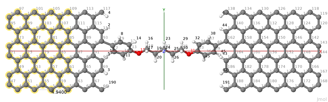
Figure 38 Jmol screenshot showing the selected contact atoms#
In Figure 38 it is possible to see the geometry
to be processed for reordering with selected atoms belonging to the first
contact.
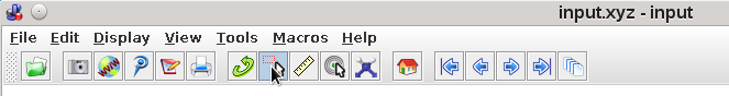
Different strategies can be used to select the contact atoms in jmol. The
easiest is probably using the select tool and use the mouse (see
Figure 39). Orient the molecule and use the
select tool by holding SHIFT + LEFT Mouse Button, then drag the mouse to include
all contact atoms (see the mouse section of the jmol wiki).
Figure 39 Jmol screenshot showing the selection tool#
NOTE: Initially, when you click on the selection tool, all atoms will be
selected and will appear highlighted. You can either
Unselect all atoms by drawing a box around the whole structure with SHIFT +
LEFT MOUSE
Choose the menu Display->Select->none to unselect all atoms.
Alternatively, open the JmolScriptConsole and type:
$ select none
Now you can select the contact atoms and then list the selected atoms by typing
into the jmol console:
$ print {selected}
In this example you will then see:
({45:6069:8493:108})
The selected atoms are shown in a compact syntax that can be directly
copy-pasted into setup_in.hsd. NOTE that this jmol command shows atom
numbers starting from 0 and not from 1. In this case use the following syntax
should be used in the setup_in.hsd input file:
Atoms[zeroBased]={45:6069:8493:108}
where the modifier zeroBased tells the code that atom indices start counting
from 0. Then repeat a similar process for the other contact.
The ContactVector specification is needed so the code can understand the
direction of the contact and the supercell periodicity. Use the measurements
tool of jmol in order to get the vector length (See
Figure 38).
The user should provide the Slater-Koster files so the code can elaborate the
correct cutoff distances. These are specified in the same way as for the DFTB+ code:
* ``SpecifiedPLs = 2``: In this case `setupgeom` reorders the second PL and
  checks that the distance between second-neighbour PLs is larger than the
  cutoff. An error is shown if this is not the case.

* ``SpecifiedPLs = 1``: In this case `setupgeom` builds as many additional PLs
  as needed to fulfil the contact requirements. This can produces thicker
  contacts with two new revised PLs.
In both cases the device region is further layered into PLs for the efficient
iterative Green’s function algorithm. In most cases the SK tables have a rather
large cutoff, extending as long as all Hamiltonian matrix elements are below
1e-5 a.u. (about 1 meV). In order to make transport calculations a little
faster it is possible to slightly shorten the SK cutoffs. A small decrease
easily results in PLs with half of the original number of atoms and hence faster
calculations, with very small effect on the final results (e.g., transmission,
ldos, currents). The SK cutoff can be set with the block TruncateSKRange
(also see the DFTB+ manual):
Clearly in doing this, accuracy is traded for speed. In the case of C-C
interactions, the parameters have a cutoff distance of about 5.17 Angstrom that
is quite comparable with a reduced cutoff of 5.0 Angstrom. In any case the user
should check and validate the results of selecting this option.
Once the input is ready, convert the structure to your preferred input file
(initial.gen in this example) and run setupgeom. As output you will find the
structure processed.gen prepared for transport calculations and a file
transport.hsd containing the Transport block needed for the following
contact calculations:
The file is formatted such that it can be appended or included into the end of
the dftb_in.hsd input.
For consistency, the user should specify exactly the same SKMaxDistance that
was used in setting up the geometry inside the input file of DFTB+ (if it is
modified from the default set by the Slater-Koster files).