Tutorial: Photoinduced charge transfer in a donor-acceptor complex.

Tutorial: Photoinduced charge transfer in a donor-acceptor complex.#

This is a tutorial given at the DFTB+ School 2022 in Daresbury, UK. The idea is to get familiar with the real-time TDDFTB method applied to molecules and molecular complexes, learning the basics of absorption spectra calculations and photoinduced processes such as charge transfer under laser irradiation. The tutorial is based on the following work: Photoinduced charge-transfer dynamics simulations in noncovalently bonded molecular aggregates. Medrano, C. R., Oviedo, M. B., and Sánchez, C. G. (2016). Physical Chemistry Chemical Physics, 18(22), 14840–14849. https://doi.org/10.1039/c6cp00231e

Spectra and analysis#

We will first calculate the absorption spectra of two different molecules and analyse them using the tools provided with DFTB+.

Calculation of the absorption spectrum of carbazole#

[Input: recipes/electronicdynamics/tutorial/01_spectra_and_laser/01_carbazole/01_spectrum]

We will calculate the absorption spectrum of the carbazole molecule, following the procedure described in Calculation of electronic absorption spectra.

Take a look at the input coordinates coords.gen. The .gen format is the one used for DFTB+ code (see section Geometry for more details). In order to visualise the molecule, you can use the gen2xyz script, provided in the installation of the DFTB+ code, by running:
```
gen2xyz coords.gen
```
This will generate a coords.xyz that you can open with VMD, Avogadro or any other molecular visualisation software of your choice. An image of the carbazole molecule made with VMD is presented in Figure 24.

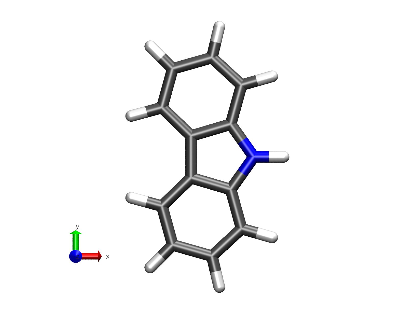
Figure 24 Carbazole molecule#
Open the dftb_in.hsd_spec file. This is a template for the calculation of the absorption spectrum.
- Take a look at the ElectronDynamics block at the end of the file:
```
 ElectronDynamics = {
     Steps =                         #define the time window
     TimeStep [au] =                 #resolution of the spectrum
     Perturbation = Kick {           #must be a kick (Dirac delta)
         PolarizationDirection =     #desired direction/s
     }
     FieldStrength [v/a] =           #Field strength of the perturbation
```
- There are four input variables to be considered for the calculation of the spectrum:
  - Steps (integer): the number of steps of the dynamics. The longer the dynamics, the lower the excitation energies that can be resolved in the spectrum (this variable affects the time taken for the simulation, but the total physical time in the simulation is also affected by value used for the TimeStep). Here, we will use 10000 steps.
  - TimeStep (float): the (physical) time a single step takes (in time units). Here we use 0.2 a.u (0.0048 fs), which is normally stable for simulations of a few tens of thousands of steps. In case there is instability in the dynamics, the time step should be decreased.
  - Perturbation: In the case of calculating a spectrum, we need a Dirac-delta perturbation (AKA kick) and we need to specify the PolarizationDirection. That could be X, Y, Z (if we are interested in one particular direction) or all if we want to calculate the three kicks consecutively and then calculate the spherically-averaged spectrum, accounting for random molecular orientations. Hence, we set it as all.
  - FieldStrength (float): strength of the electric field of the perturbation being applied. For the calculation of the absorption spectrum, it must be within the linear response regime, i.e., usually 0.001 \(V/Å\) or lower.
- Complete the template file, copy it to dftb_in.hsd and run the calculation.
Once the dynamics ends, we will have calculated the time-resolved dipole moment using three different field polarisation directions (mux.dat, muy.dat, muz.dat). We need to average and Fourier-transform (or the other way around, as these are linear operations) these dipole components in order to obtain the absorption spectrum of the molecule. To do this, we will use the calc_timeprop_spectrum tool available after installation of DFTB+ under: dftbplus/tools/misc/. In the folder where you have the dipole files just type:
```
calc_timeprop_spectrum -d 4 -f 0.001
```
where the option -d is for the damping constant (artificial lifetime, in fs), which is equivalent to convoluting each resonance with a Lorentzian in time domain. The option -f is the field strength of the kick (in \(V/Å\)) applied during dynamics.
After running the script you will find two new files: spec-nm.dat and spec-ev.dat which are the absorption spectra in nm and eV, respectively. Plot the spectrum file with the plotting tool of your choice and look at the lowest energy transitions. You should then see an absorption spectrum similar to Figure 25.

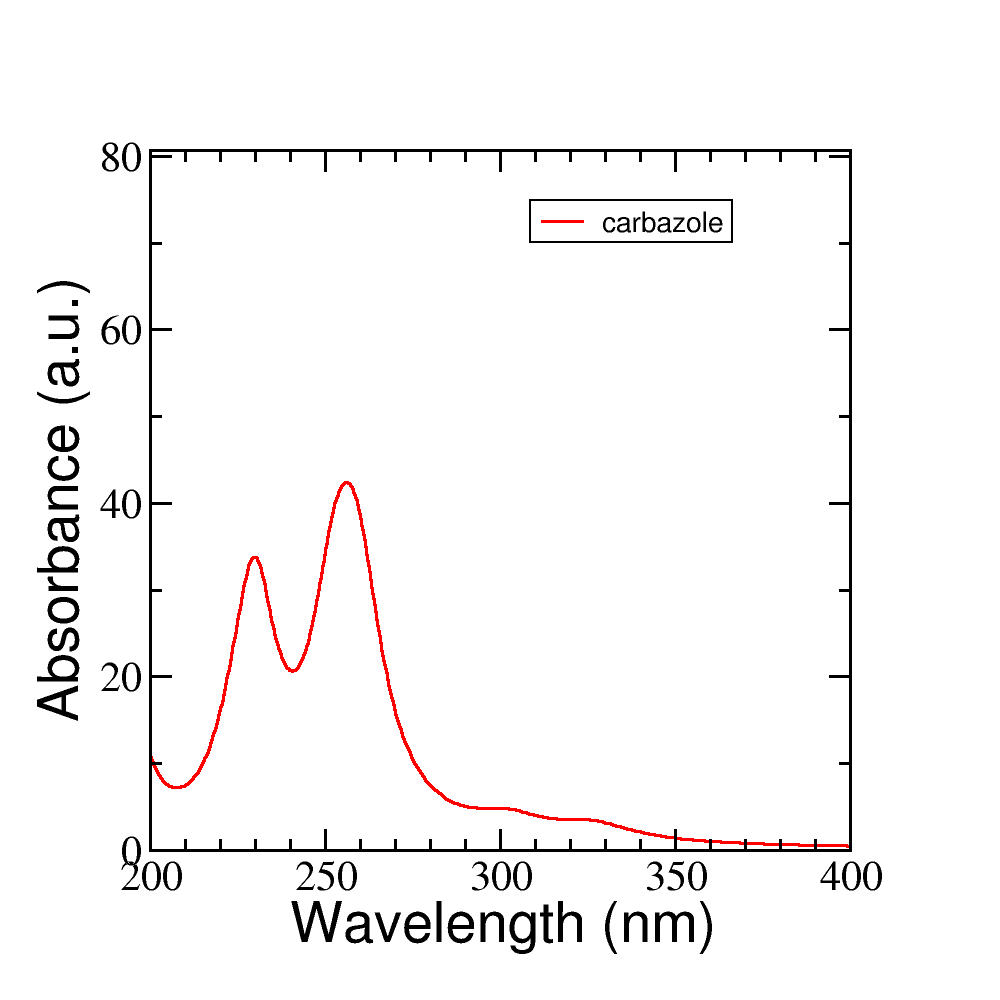
Figure 25 Absorption spectrum of carbazole molecule#
Change the damping constant for a higher value, recalculate the spectrum and plot both spectra together. What is the effect of the damping time on the spectrum? Figure Figure 26 shows the same spectrum calculated with different values of the damping constant.

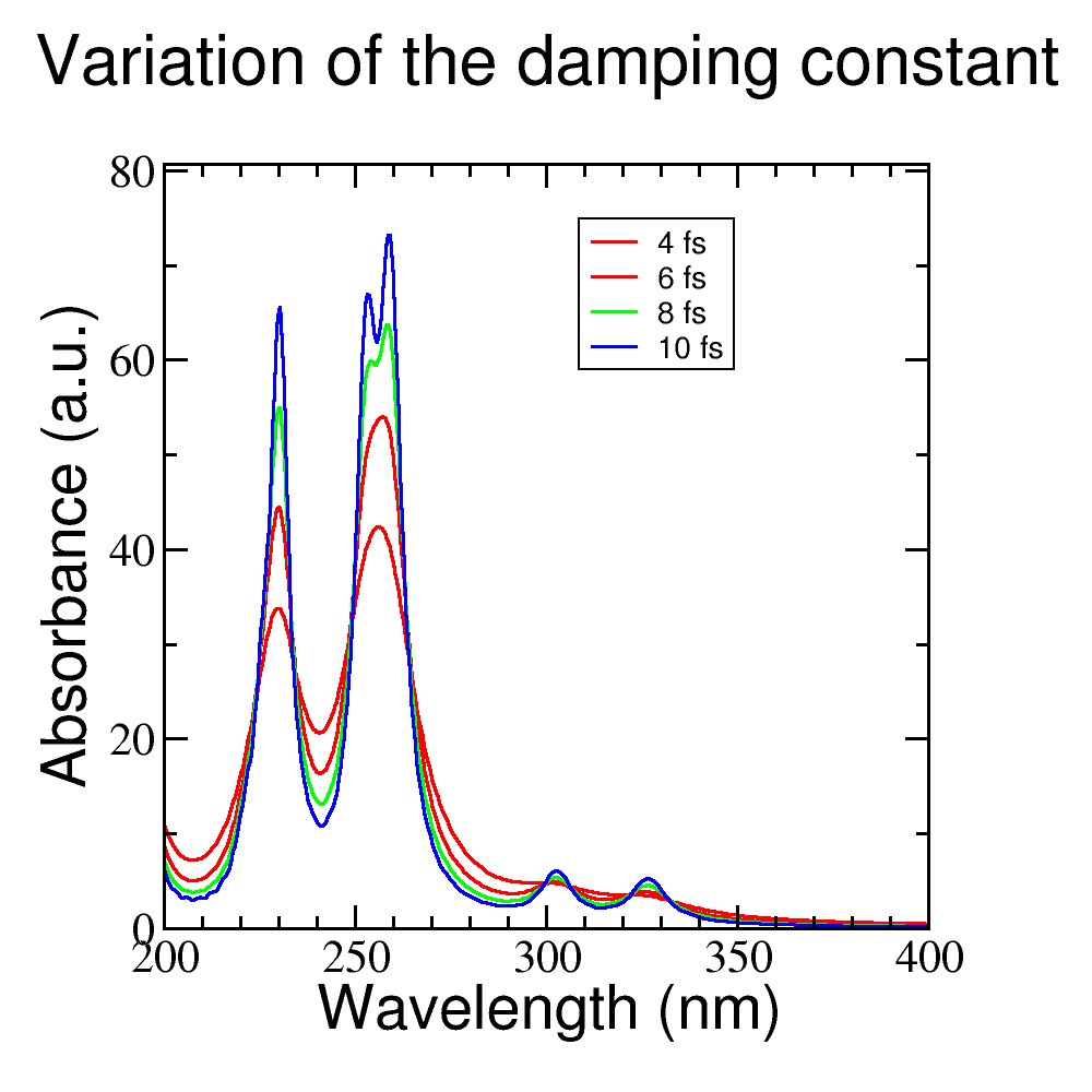
Figure 26 Influence of the damping constant value d in the absorption spectrum.#

Analysis of the absorption spectrum of carbazole: driving the system with a laser#

[Input: recipes/electronicdynamics/tutorial/01_spectra_and_laser/01_carbazole/02_laser]

We will consider a laser perturbation in resonance with the lowest energy transition of the molecule in order to study the photodynamic process of absorption by this transition. In order to do this, we will follow the same procedure as described in Driving electronic dynamics with external fields, first finding the lowest energy dipole-allowed transition of the molecule in from spectrum plotted in the previous calculation, and then calculating the direction of maximal polarisation of the transition.

Open the dftb_in.hsd_laser file. This is a template for the calculation of a laser perturbation.
- Take a look at the ElectronDynamics block at the end of the file:
```
  Scc = Yes
  SccTolerance = 1e-7  
  MaxAngularMomentum {
    C = "p"
    H = "s"
    N = "p"
  }
  SlaterKosterFiles = Type2FileNames {
    Prefix = "../../../../slakos/download/mio-1-1/"
    Separator = "-"
```
  Here, the Perturbation type is a continuous-wave laser, for which we need to specify two parameters:
  - LaserEnergy (float): the photon energy of the laser being applied to excite transition energy of interest. This value must be in energy units, like eV, or with wavelength units such as nm.
  - PolarizationDirection (vector): in the case of a laser, the PolarizationDirection is a 3-components vector.
  Note that we turned on the Populations flag in order to write the orbital occupations during the dynamics. Also note that we are asking for the detailed xml and the eigenvectors with the WriteDetailedXML and WriteEigenvectors options. We will need them to plot the orbitals with waveplot in the following sections.
To complete the input template for the laser, we need to provide the LaserEnergy and the PolarizationDirection of the light. Based on our previous calculated spectrum, calculate the direction of maximal polarisation of the lowest energy transition of the molecule.
- Help: use the tool calc_timeprop_maxpoldir already available in your installation (under: dftbplus/tools/misc/). To know how this tool work the user can just type:
```
calc_timeprop_maxpoldir -h
```
- Along which axis/axes is the polarisation of the molecule oriented? Why?
  - Hint: try to visualise the molecule and see how it is oriented with respect to the cartesian axes.
- Solution: If you choose the lower energy transition of carbazole you may do:
```
calc_timeprop_maxpoldir -10 -w 326
```
  and you will obtain the following transition dipole vector:
```
PolarizationDirection = 0.99999 0.00101 -0.003815
```
  which is essentially parallel to the X cartesian direction (because of the molecule’s orientation).
Prepare the input for the dynamics under a continuous laser perturbation. Use the energy obtained from the spectrum as the LaserEnergy and the most polarisable direction obtained above for the PolarizationDirection of the laser.
- Why we should use this laser polarisation, instead of any other type of perturbation?
After the dynamics, take a look at the mu.dat file. You could plot the 3 components of the dipole moment by doing:
```
xmgrace -nxy mu.dat
```
In Figure 27 the dipole moment is plotted.
- Is the dipole moment increasing linearly?
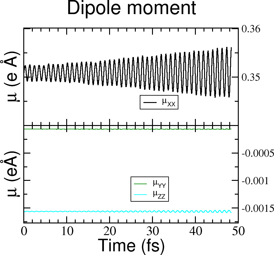
Figure 27 Dipole moment components vs time for the laser dynamics.#
Take a look at the molpopul1.dat file generated. This file contains the populations projected on the ground-state (GS) orbitals during the dynamics:
```
# GS molecular orbital populations, spin channel : 1
#time (fs) | population (orb 1) | population (orb 2) | ... | population (orb N) |
0.237050663997490  1.999999999825206  1.999999999780047  1.999999999771997  ...
0.478939096647990  1.999999999978780  1.999999999983538  1.999999999962606  ...
0.720827529298490  1.999999999870651  1.999999999913354  1.999999999904491  ...
```
- Which orbitals are involved in the transition? Help: you can plot the molpopul1.dat file using xmgrace:
```
xmgrace -nxy molpopul1.dat
```
  Look at the populations initially at y=2 (occupied orbitals in the GS basis) and find which curves are decreasing over time, these are the orbitals being depopulated. Look at the populations initially at y=0 (unoccupied orbitals in the GS basis) and find the orbitals being populated over time.
  
  You could also check in the band.out file generated from the SCC calculation the state numbers. Close to the Fermi energy, you should see something like:
```
29    -6.641  2.00000
30    -5.809  2.00000
31    -5.512  2.00000    #HOMO
32    -1.983  0.00000    #LUMO
33    -1.358  0.00000
34    -0.501  0.00000
```
  where it is clear that states 31 and 32 are the HOMO and LUMO of the molecule, respectively.
Let’s visualise those orbitals using waveplot. For a complete description please check First steps with Waveplot.
- Look at the waveplot_in.hsd_ template input file for waveplot:
  - Which files are needed?
  - In which orbitals are we interested?
- After editing this file, just rename it to waveplot_in.hsd and run waveplot using your current installed executable, which should be in the same installation directory as the dftbplus executable.
- After running waveplot, a number of files would be generated starting with “wp-1-1”.
Let’s plot these orbitals:
- Open the cube files that correspond to the HOMO and LUMO and plot them as an isosurface. For that there are several software options. Particularly, we give here some links for VMD and VESTA: For a tutorial on the Basics of VMD and/or plotting an isosurface method please refer to these links. VESTA allows the user to open directly cube files showing the isosurface immediately with some default parameters, making it a really good option for quick inspections.

As a reference, we plotted the populations obtained from the laser dynamics and the orbitals involved in the transition in Figure 28.

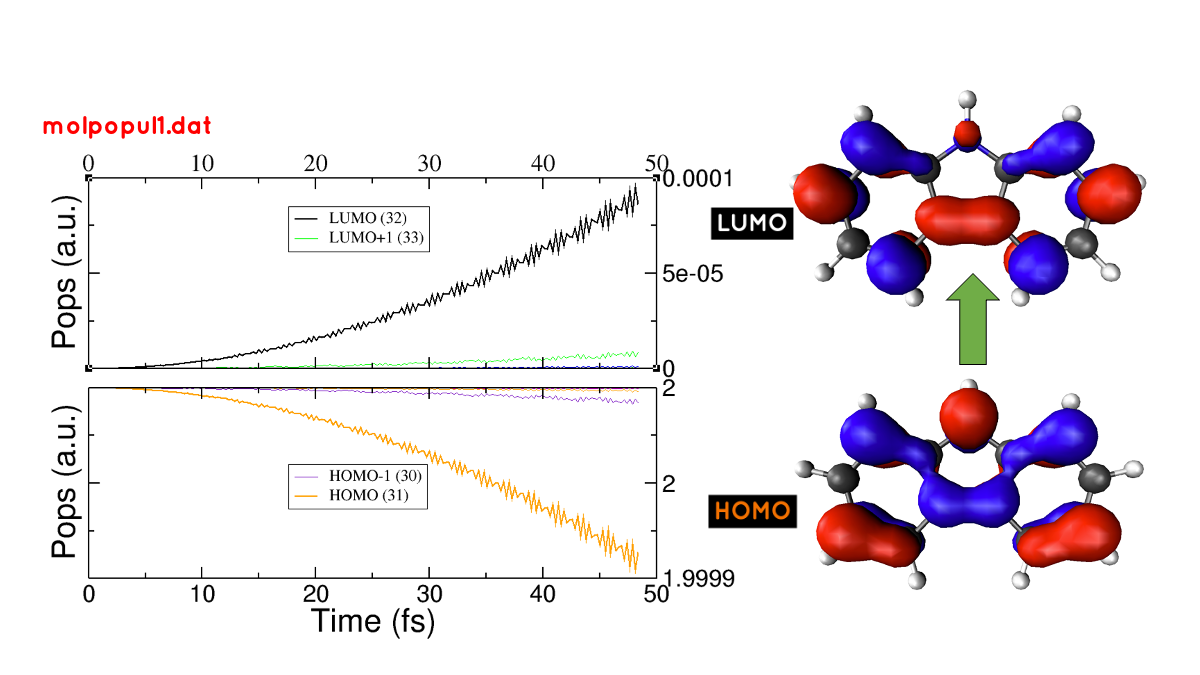
molpopul1-carbazole — Figure 28 (left) Populations vs time for the laser dynamics. (right) Orbitals involved in the lower energy transition of the carbazole molecule.#

Now it’s your turn!

Calculation of PDI absorption spectrum#

[Input: recipes/electronicdynamics/tutorial/01_spectra_and_laser/02_PDI/`]

We will repeat the procedure used for the carbazole molecule with a new molecule, PDI.

Based on the calculations that you ran before.
- Calculate the absorption spectrum with a proper dftb_in.hsd input file.
- Find the lowest energy transition.
- Apply a laser tuned with this transition.
- Obtain the orbitals involved in the transition using waveplot and plot them.

The reference results are plotted in Figure 29

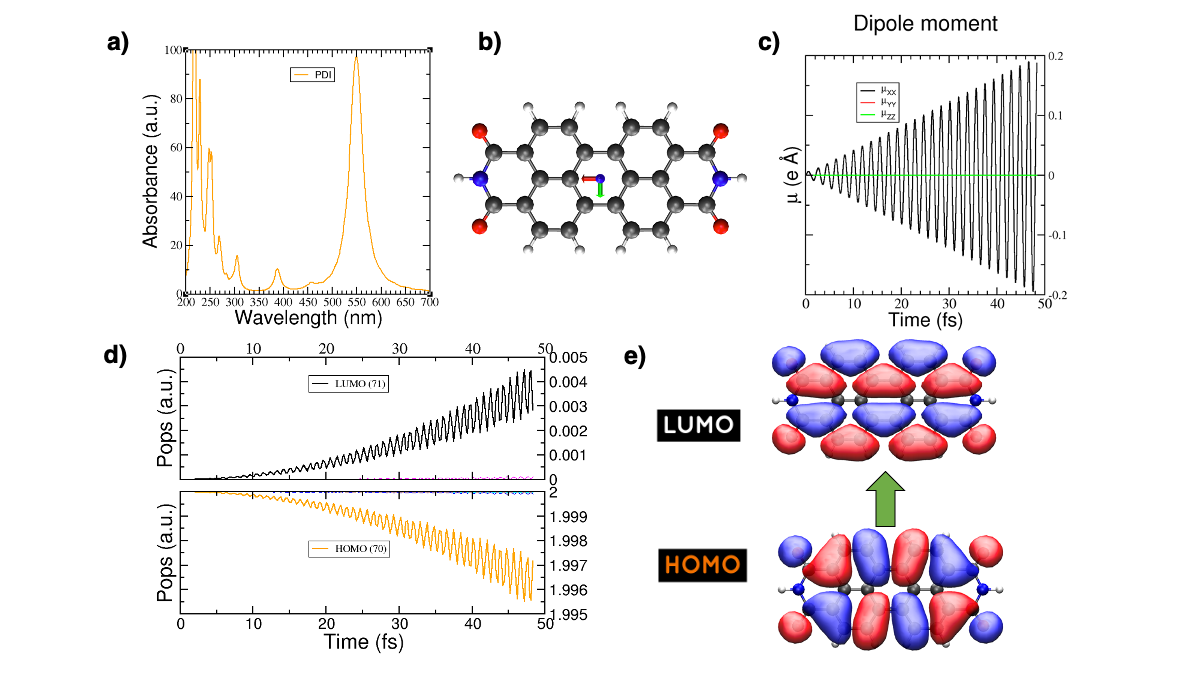
Figure 29 (a) Absorption spectrum of the PDI molecule. (b) PDI molecule structure. (c) Dipole moment components vs time during a laser dynamics at 548 nm (note that in this case the dipole moment in the X direction increases linearly). (d) Populations vs time for the laser dynamics. (e) Orbitals involved in the transition.#

Photoinduced charge transfer#

Calculate the absorption spectrum of a donor-acceptor aggregate#

[Input: recipes/electronicdynamics/tutorial/02_photoinduced_CT/01_aggregate_spec/]

Visualise the coordinates file coords.xyz.

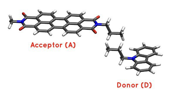
Figure 30 PDI+carbazole derivatives aggregate#

It is an aggregate of the two previous molecules, in which the carbazole and PDI derivatives act as donor and acceptor of electrons, respectively.

Convert the coordinates into gen format (using the xyz2gen script) and calculate the absorption spectrum using the dftb_in.hsd_spec as a template for the input (copy this file or rename it as dftb_in.hsd).

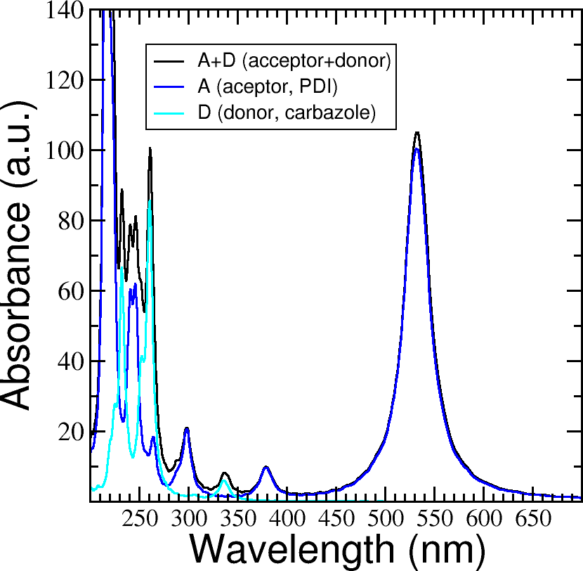
Note that after the electron dynamics, you will need (as before) to run the Fourier transform of the induced dipole moment of the system (using the calc_timeprop_spectrum tool) in order to obtain the spectrum.
Compare the calculated spectrum with the individual ones (you can use the spectra calculated before or recalculate them from these derivatives). For the comparison to be valid, you should use the same damping constant for all spectra. Are there relevant differences? See Figure 31.

Figure 31 Absorption spectrum of the PDI+carbazole derivatives aggregate (in black), compared to the individual spectrum for the PDI moiety (in blue) and the carbazole moiety (in teal).#
We are interested in the dynamics upon illumination of the acceptor molecule. For such purpose, we will perform a driven simulation in next step and for it, we need to calculate the transition dipole direction of the absorption band at ~530 nm. Calculate this vector using the calc_timeprop_maxpoldir tool. You should obtain something similar to:
```
PolarizationDirection = -0.99977 0.01777 0.01122
```
which is essentially the X direction (since the PDI molecule axis is parallel to the X axis in the coordinates).

Laser dynamics on the donor-acceptor aggregate and charge transfer#

[Input: recipes/electronicdynamics/tutorial/02_photoinduced_CT/02_aggregate_CT/]

With the transition dipole moment vector calculated previously, prepare your input file for a laser-driven electron dynamics in tune with the acceptor (PDI) lowest energy excitation. Use the dftb_in.hsd_pulse as a template. Note that this time we add an envelope function to the laser perturbation in order to mimic a laser pulse:
```
  Scc = Yes
  SccTolerance = 1e-7  
  MaxAngularMomentum {
    C = "p"
    H = "s"
    N = "p"
    O = "p"
  }
  SlaterKosterFiles = Type2FileNames {
    Prefix = "../../../slakos/download/mio-1-1/"
    Separator = "-"
    Suffix = ".skf"
  }
>>>>>>> 24252cf (Make formal changes)
}
```
Now in the ElectronDynamics we added the Sin2 choice for EnvelopeShape, with a duration of 30 fs starting at the beginning of the dynamics. We will also ask the code to print the populations during dynamics to study the mechanism of charge transfer. Complete the input template filling the PolarizationDirection and LaserEnergy obtained before and run the code (don’t forget to rename the template to dftb_in.hsd).
After running the electron dynamics, let inspect the qsvst.dat file
```
#time (fs) | total net charge (e) | charge (atom_1) (e) | ... | charge (atom_N) (e)|
0.000000000000000   -0.000000000000055   0.075753114169209   0.077680106829215  ...
0.241888432650500   -0.000000000000048   0.075753940652948   0.077680933651269  ...
0.483776865301000   -0.000000000000049   0.075758821681684   0.077685768802125  ...
```
The first column of the file is the time and the second one is the total net charge of the system at each time step (which should be always close to zero, within numerical error). After that, the next columns are the net atomic charges at each time step. Making use of the file qsvst.dat one may potentially get information about partial charge motion during dynamics. If you are interested in what is happening with the charge of one molecule in your system, you can sum the over the atomic charges of the atoms of that molecule to get the evolution of the net molecular charge over time.
As we are interested in the charge transfer between both molecules we want to analyse the net charge of each molecule during the dynamics. For this purpose, you could write your own script but we also provide you with a simple script which works fine for this case. The provided tool calc_timeprop_charges.py, which you can find in the same directory as the template input file, will do the job.

Try
```
./calc_timeprop_charges.py --help
```
to get info about how to use the script
```
usage: calc_timeprop_charges.py -l ii:jj,ll:mm

Reads output from TD calculation with external laser and produces net charges per fragment
(subtracting value at time = 0).

Needs qsvst.dat file present in working directory.

Options:
-h, --help            show this help message and exit
-l AT_LIST, --list=AT_LIST
                  list of atom indices starting from 1 (initial and
                  final index separated by colons, ranges separated by
                  commas)
```
You will have to define the ranges of atoms that correspond to each of the two molecules. In our case, the PDI derivative is between atom 1 and 52 and the carbazole derivative is between atom 53 and 83. Then, you may run:
```
./calc_timeprop_charges.py -l 1:52,53:83
```
After running the script, two files may be generated: charge_frag1.dat and charge_frag2.dat with the corresponding charges of each defined fragment. If you plot it you will get something like Figure 32.

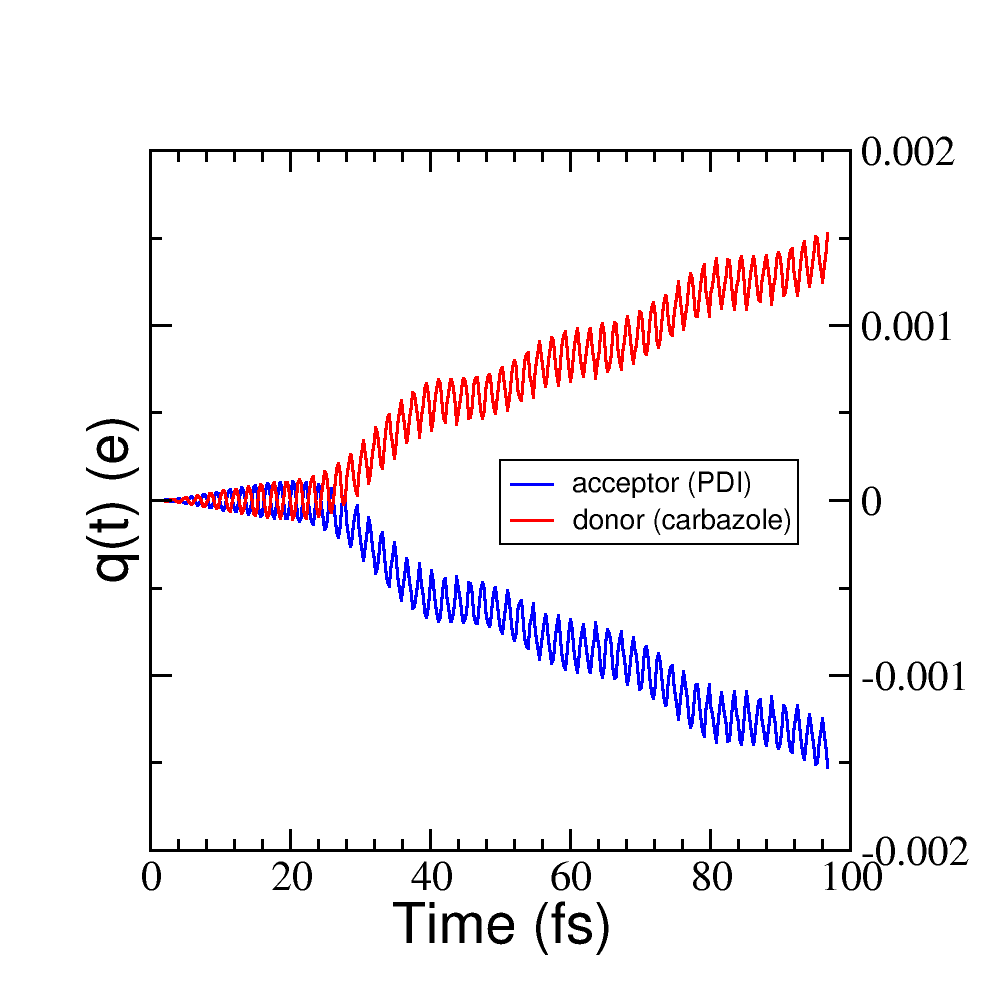
Figure 32 Charge vs time for the acceptor and donor molecules.#

where it is clear that the PDI molecule act as an acceptor of electrons (net charge goes negative), while the carbazole is donating electrons (net charge goes positive).

If we follow the protocol from before, ploting the populations and searching for the orbitals involved in the transition, we should be able to get some insights into the mechanism of the charge transfer (follow the steps in the previous sections). As it is shown in Figure 33.

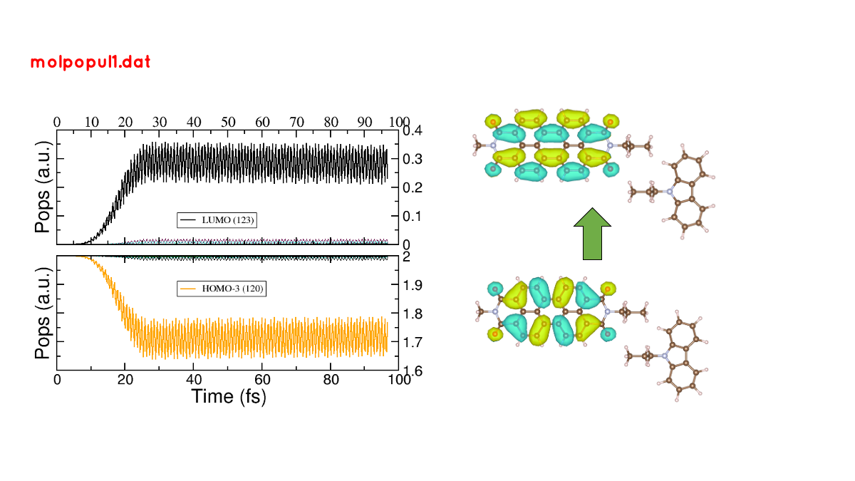
Figure 33 (left) Populations vs time for pulse-driven dynamics. (right) Orbitals involved in the excitation during the dynamics.#

the orbitals involved in the excitation with the pulse are localised in the PDI molecule, i.e., we can confirm that we are exciting the PDI molecule via it’s HOMO-LUMO transition (and not the HOMO-LUMO transition of the whole system). Comparing with the previous figure of the charges dynamics, we can also see that the CT process start after a certain amount of electrons are excited in the PDI molecule (more or less 30 fs, the duration of the pulse used). So we could in principle divide the mechanism into two steps. The first one, from 0 to ~30 fs where the PDI is being excited. The second step is the charge transfer from the carbazole to the PDI once the latter is already excited.

We hope that this tutorial is helpful for those interested in get into the real-time TDDFTB method using DFTB+. Of course, these are just the basics and there are many more possibilities in terms of calculating optical properties and photoinduced processes within this approach for a wide range of materials and system like graphene nanoribbons, plasmonic nanoparticles, gold nanoclusters, semiconductor nanoparticles and organic solar cells. As an inspiration, we give you some references of some recent works performed with this method in DFTB+:

Fano Resonance and Incoherent Interlayer Excitons in Molecular van der Waals Heterostructures. Lien-Medrano, C. R., Bonafé, F. P., Yam, C. Y., Palma, C.-A., Sánchez, C. G., and Frauenheim, T. (2022). Nano Letters, 22(3), 911–917. https://doi.org/10.1021/acs.nanolett.1c03441

Dynamical evolution of the Schottky barrier as a determinant contribution to electron-hole pair stabilization and photocatalysis of plasmon-induced hot carriers. Berdakin, M., Soldano, G., Bonafé, F. P., Liubov, V., Aradi, B., Frauenheim, T., and Sánchez, C. G. (2022). Nanoscale, 14(7), 2816–2825. https://doi.org/10.1039/d1nr04699c

Photoinduced charge-transfer in chromophore-labeled gold nanoclusters: quantum evidence of the critical role of ligands and vibronic couplings. Domínguez-Castro, A., Lien-Medrano, C. R., Maghrebi, K., Messaoudi, S., Frauenheim, T., and Fihey, A. (2021). Nanoscale, 13(14), 6786–6797. https://doi.org/10.1039/D1NR00213A

Plasmon-driven sub-picosecond breathing of metal nanoparticles. Bonafé, F. P., Aradi, B., Guan, M., Douglas-Gallardo, O. A., Lian, C., Meng, S., Frauenheim, T., and Sánchez, C. G. (2017). Nanoscale, 9(34), 12391–12397. https://doi.org/10.1039/C7NR04536K